API reference

API reference#

\(\mathrm{LiMe}\) features a composite software design, utilizing instances of other classes to implement the target functionality. This approach is akin to that of IRAF: Functions are organized into multi-level packages, which users access to perform the corresponding task. The diagram below outlines this workflow:

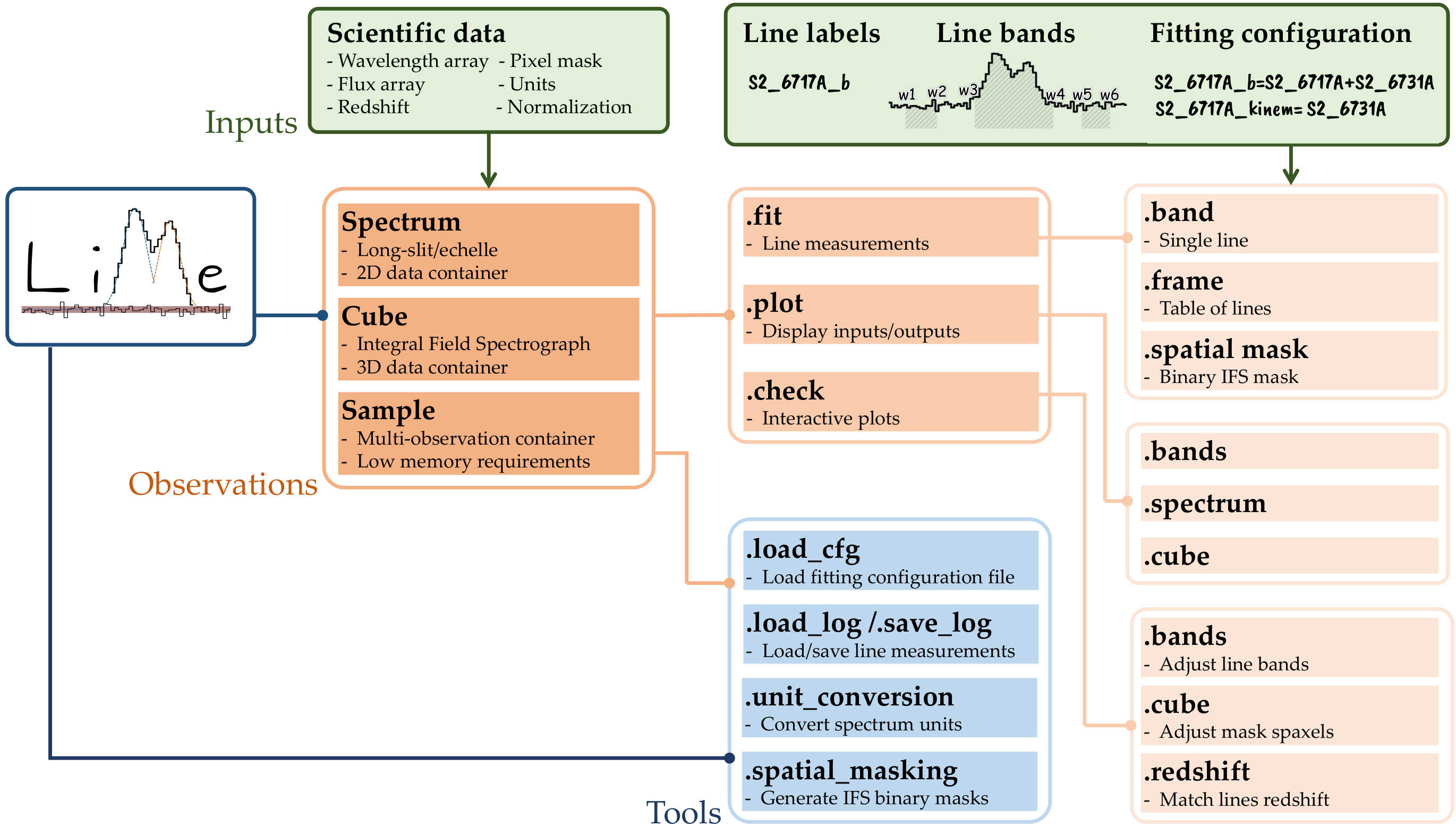
At the highest level, \(\mathrm{LiMe}\) provides of observational classes: spectrum, cube, and sample. The first two are essentially 2D and 3D data containers, respectively. The third class functions as a dictionary-like container for multiple spectrum or cube objects. Moreover, as illustrated in the figure above, various tools can be invoked via the \(\mathrm{LiMe}\) import for tasks, such as loading and saving data. Many of these functions are also within the observations.

At an intermediate level, each observational class includes the .fit, .plot, and .check objects. The first provides functions to launch the measurements from the observation data. The second organizes functions to plot the observations and/or measurements, while the emph{.check} object facilitates interactive plots, allowing users to select or adjust data through mouse clicks or widgets. In these functions, users must specify an output file to store these user inputs.

Finally, at the lowest level, we find the functions that execute the measurements or plots. Beyond the aforementioned functionality, the main distinction between these commands lies in the extent of the data they handle.

For instance, the Spectrum.fit.bands and Spectrum.fit.frame commands fit a single line and a list of lines in a spectrum, respectively. Conversely, the Cube.fit.spatial_mask command fits a list of lines within a spatial region of an IFS cube.

The next sections detail the functions attributes and their outputs:

Information#

lime.show_instrument_cfg()[source]

Display the available instrument configurations for LiMe FITS observations.

The information is printed to the console for user inspection.

Return type:: None

Notes

Each entry includes:
- units_wave — wavelength units
- units_flux — flux units
- pixel_mask — mask handling flag
- res_power — instrumental resolving power

Examples

Display all supported instrument configurations:

>>> show_instrument_cfg()

Example output:

Long-slit “.fits” observation instrument configuration: 0 osiris) units_wave: Angstrom, units_flux: erg/s/cm2/A, pixel_mask: False, res_power: 5000

Cube “.fits” observation instrument configuration: 0 megaracube) units_wave: Angstrom, units_flux: erg/s/cm2/A, pixel_mask: True, res_power: 6000

lime.show_profile_parameters(profile_params={'e': ['amp', 'center', 'alpha'], 'g': ['amp', 'center', 'sigma'], 'l': ['amp', 'center', 'sigma'], 'p': ['a', 'b', 'c', 'alpha'], 'pp': ['amp', 'center', 'sigma', 'alpha', 'frac'], 'pv': ['amp', 'center', 'sigma', 'frac'], 'v': ['amp', 'center', 'sigma', 'gamma']}, profile_abbrev={'e': 'Exponential', 'g': 'Gaussian', 'l': 'Lorentzian', 'p': 'Broken Power law', 'pp': 'Pseudo-Power law', 'pv': 'Pseudo-Voigt', 'v': 'Voigt'})[source]

Display the available emission line profile models and their parameters.

Parameters:

profile_params (dict, optional) – Dictionary mapping profile identifier characters (e.g., "g", "l") to lists of parameter names (e.g., ["amplitude", "center", "sigma"]). Default is PROFILE_PARAMS.
profile_abbrev (dict, optional) – Dictionary mapping profile identifier characters to their descriptive names (e.g., {"g": "Gaussian", "l": "Lorentzian"}). Default is PROFILE_ABBREV.

Examples

Display all registered profiles:

>>> show_profile_parameters()

Example output:

Available profiles (with their identifying character) and their parameters:
- Gaussian "g": ['amp', 'center', 'sigma']
- Lorentzian "l": ['amp', 'center', 'sigma']
- Voigt "v": ['amp', 'center', 'sigma', 'gamma']

Inputs/outputs#

lime.load_cfg(file_address, fit_cfg_suffix='_line_fitting')[source]

Load a LiMe configuration file (TOML) and normalize LiMe-specific sections.

This reads a TOML configuration file and, for any section whose name ends with fit_cfg_suffix, converts its key/value pairs to the formats expected by LiMe’s line-fitting routines.

Parameters:

file_address (str or pathlib.Path) – Path to the input configuration file (.toml).
fit_cfg_suffix (str, optional) – Section-name suffix that identifies LiMe line-fitting configuration blocks to be normalized. Default is "_line_fitting".

Returns:

Parsed configuration mapping with LiMe sections converted where applicable.

Return type:

dict

Raises:

LiMe_Error – If the file does not exist at file_address.
tomllib.TOMLDecodeError – If the TOML file cannot be parsed.

Notes

Sections ending with fit_cfg_suffix are passed to parse_lime_cfg for normalization.
If an item within a fit_cfg_suffix section cannot be converted, a critical warning is emitted (handled inside parse_lime_cfg), but the rest of the configuration is still returned when possible.
Requires Python 3.11+ for tomllib.

Examples

>>> cfg = load_cfg("settings.toml")
>>> cfg["my_model_line_fitting"]["method"]
'gaussian'

lime.load_frame(fname, page: str = 'FRAME', levels: list = ['id', 'line'])[source]

Loads a lines frame (pandas.DataFrame) from various file formats.

Supported inputs include plain text tables, CSV, FITS HDUs, Excel sheets, ASDF nodes, and Streamlit UploadedFile objects. If the resulting table contains the columns listed in levels, a MultiIndex is reconstructed by setting those columns as the index.

Parameters:

fname (str or pathlib.Path or UploadedFile) – Path to the lines log file or a Streamlit UploadedFile. When a path is provided, the file type is inferred from the suffix.
page (str, optional) – HDU name (FITS) / sheet name (Excel) / node key (ASDF) to read from. Used only for .fits, .xlsx/.xls, and .asdf inputs. Default is "FRAME".
levels (list of str, optional) – Column names to use for reconstructing a MultiIndex via DataFrame.set_index. If all names in levels are present as columns, they are set as the index. Default is ["id", "line"].

Returns:

The loaded lines log. For text/CSV/Excel/ASDF the first column is treated as the initial index during read; if all levels are present as columns, they are set as a MultiIndex on return.

Return type:

pandas.DataFrame

Raises:

LiMe_Error – If fname is a path and the file does not exist.
SystemExit – If the file exists but cannot be opened/parsed (wraps a ValueError).

Notes

Detected formats and readers:

.fits: read via hdu_to_log_df(log_path, page).
.xlsx / .xls: read via pandas.read_excel(..., sheet_name=page, header=0, index_col=0).
.asdf: read node page and build a DataFrame from records; index set from the "index" field.
.txt: whitespace-separated via pandas.read_csv(..., sep=r"\s+", header=0, index_col=0, comment="#").
.csv: comma-separated via pandas.read_csv(..., sep=",", header=0, index_col=0, comment="#").
UploadedFile (Streamlit): treated like a whitespace-separated text table.

Examples

Load an Excel sheet named FRAME and restore a MultiIndex of (id, line):

>>> df = load_frame("lines.xlsx", page="FRAME", levels=["id", "line"])

Load a FITS HDU named FRAME:

>>> df = load_frame("lines.fits", page="FRAME")

lime.save_frame(fname, dataframe, page='FRAME', parameters='all', header=None, column_dtypes=None, safe_version=True, **kwargs)[source]

Save a lines frame (pandas.DataFrame) to disk in one of several supported formats.

The output format is inferred from the file extension. Supported formats include plain text tables, FITS HDUs, ASDF trees, and Excel sheets. Optional metadata such as FITS/ASDF headers and custom column data types can be provided.

Parameters:

fname (str or pathlib.Path) – Destination file path. The extension determines the file format. Supported extensions are .txt, .fits, .asdf, and .xlsx.
dataframe (pandas.DataFrame) – Lines log to be saved.
parameters (list or {"all"}, optional) – Columns to include in the output. If "all", all DataFrame columns are written. Default is "all".
page (str, optional) – HDU name (for FITS) or sheet name (for Excel) to use when writing. Default is "FRAME".
header (dict, optional) – Additional metadata to include in the output file. For FITS and ASDF files, this dictionary is added to the file header.
column_dtypes (str, type, or dict, optional) – Data type conversion mapping for the output FITS record array. - If a string or type, all columns are cast to that type. - If a dictionary, specify a mapping of column names or indices (zero-indexed) to their desired data types. This argument overrides LiMe’s default FITS formatting.
safe_version (bool, optional) – If True, the current LiMe version is saved as a footnote or page header in the output log. Default is True.

Raises:

ValueError – If the file extension is unsupported or the DataFrame cannot be written in the specified format.

Notes

For FITS and Excel outputs, the target HDU or sheet is named according to page.
FITS headers can be extended using header.
Custom column data types can be enforced via column_dtypes.
The function ensures compatibility with LiMe’s internal data formats.

Examples

Save a DataFrame to a FITS file with a custom header:

>>> header = {"OBSERVER": "V. Pérez", "INSTRUME": "MEGARA"}
>>> save_frame("lines.fits", df, header=header)

Save selected columns to an Excel sheet named FRAME:

>>> save_frame("lines.xlsx", df, parameters=["profile_flux", "profile_flux_err", "eqw"], page="FRAME")

Loading long-slit .fits files#

lime.OpenFits.osiris(fits_address, data_ext_list=0, hdr_ext_list=0, **kwargs)

Load spectral data and metadata from an OSIRIS FITS observation.

The function extracts the wavelength, flux, and (if available) uncertainty arrays from the specified FITS file. It also returns the selected header(s) and a dictionary of LiMe Spectrum parameters describing the observation units, normalization, and WCS configuration.

Parameters:

fits_address (str or pathlib.Path) – Path to the OSIRIS observation FITS file.
data_ext_list (int, str, or list of {int, str}, optional) – Extension(s) containing the spectral data. Each element may be an integer index or an extension name. Default is 0.
hdr_ext_list (int, str, or list of {int, str}, optional) – Extension(s) containing the FITS headers corresponding to the data extensions. Each element may be an integer index or an extension name. Default is 0.
**kwargs – Additional keyword arguments passed to load_fits().

Returns:

wave_array (ndarray of shape (n,)) – Wavelength array reconstructed from FITS header keywords CRVAL1, CD1_1, and NAXIS1.
flux_array (ndarray of shape (n,)) – Flux values from the FITS data extension.
err_array (ndarray of shape (n,), optional) – Flux uncertainty array, if available. Returned as None if no uncertainty extension is found.
header_list (list of astropy.io.fits.Header) – Headers corresponding to the selected data extensions.
params_dict (dict) – Observation parameters required to initialize a LiMe Spectrum, including wavelength/flux units, normalization, and WCS information.

Notes

The function assumes a linear wavelength solution defined by FITS header keywords CRVAL1, CD1_1, and NAXIS1.
For two-dimensional FITS data arrays (shape == (2, n)), the first row is interpreted as flux and the second as uncertainty.
For one-dimensional arrays, only the flux is returned and err_array is None.

Examples

Load an OSIRIS FITS file and retrieve its spectral arrays:

>>> wave, flux, err, hdrs, params = osiris("osiris_obs.fits")

Load a specific data and header extension by name:

>>> wave, flux, err, hdrs, params = osiris("osiris_obs.fits",
...                                        data_ext_list="SCI",
...                                        hdr_ext_list="SCI_HDR")

Loading long-slit .text files#

lime.OpenFits.text(file_address, **kwargs)

Load a spectrum from a plain text file.

This function reads a spectral table from a text file, unpacks the wavelength and flux columns, and optionally extracts uncertainty and pixel mask data if present.

Commented lines (for example #units_flux: FLAM) at the end of the document are parsed as arguments for the lime.Spectrum.Spectrum function.

Parameters:

file_address (str or pathlib.Path) – Path to the text file containing the spectrum.
**kwargs – Additional keyword arguments passed directly to [numpy.loadtxt](https://numpy.org/doc/stable/reference/generated/numpy.loadtxt.html), such as delimiter, comments, or skiprows.

Returns:

wave_array (ndarray of shape (n,)) – Wavelength array.
flux_array (ndarray of shape (n,)) – Flux values.
err_array (ndarray of shape (n,), optional) – Flux uncertainties if available (third column). None if not provided.
header_list (None) – Placeholder for compatibility with other readers; always None for text input.
params_dict (dict) –
Dictionary containing spectrum metadata such as:
- redshift : float, optional
- norm_flux : float, optional
- id_label : str, optional
- pixel_mask : ndarray, optional
These parameters are extracted from the comment section or inferred from the file content.

Notes

If the text file follows the format produced by lime.Spectrum.retrieve.spectrum(), the function automatically recovers the wavelength and flux units, flux normalization, and redshift values stored in the file header.
The function supports files with up to four columns:
1. Wavelength
2. Flux
3. Uncertainty (optional)
4. Pixel mask (optional)

Examples

Load a simple two-column spectrum file:

>>> wave, flux, err, hdr, params = lime.OpenFits.text("spectrum.txt")

Load a spectrum with custom delimiters using numpy.loadtxt options:

>>> wave, flux, err, hdr, params = lime.OpenFits.text("spectrum.dat", delimiter=",", skiprows=2)

Loading long-slit .fits files#

lime.OpenFits.text(file_address, **kwargs)

Load a spectrum from a plain text file.

This function reads a spectral table from a text file, unpacks the wavelength and flux columns, and optionally extracts uncertainty and pixel mask data if present.

Commented lines (for example #units_flux: FLAM) at the end of the document are parsed as arguments for the lime.Spectrum.Spectrum function.

Parameters:

file_address (str or pathlib.Path) – Path to the text file containing the spectrum.
**kwargs – Additional keyword arguments passed directly to [numpy.loadtxt](https://numpy.org/doc/stable/reference/generated/numpy.loadtxt.html), such as delimiter, comments, or skiprows.

Returns:

wave_array (ndarray of shape (n,)) – Wavelength array.
flux_array (ndarray of shape (n,)) – Flux values.
err_array (ndarray of shape (n,), optional) – Flux uncertainties if available (third column). None if not provided.
header_list (None) – Placeholder for compatibility with other readers; always None for text input.
params_dict (dict) –
Dictionary containing spectrum metadata such as:
- redshift : float, optional
- norm_flux : float, optional
- id_label : str, optional
- pixel_mask : ndarray, optional
These parameters are extracted from the comment section or inferred from the file content.

Notes

If the text file follows the format produced by lime.Spectrum.retrieve.spectrum(), the function automatically recovers the wavelength and flux units, flux normalization, and redshift values stored in the file header.
The function supports files with up to four columns:
1. Wavelength
2. Flux
3. Uncertainty (optional)
4. Pixel mask (optional)

Examples

Load a simple two-column spectrum file:

>>> wave, flux, err, hdr, params = lime.OpenFits.text("spectrum.txt")

Load a spectrum with custom delimiters using numpy.loadtxt options:

>>> wave, flux, err, hdr, params = lime.OpenFits.text("spectrum.dat", delimiter=",", skiprows=2)

lime.show_instrument_cfg()[source]

Display the available instrument configurations for LiMe FITS observations.

The information is printed to the console for user inspection.

Return type:: None

Notes

Each entry includes:
- units_wave — wavelength units
- units_flux — flux units
- pixel_mask — mask handling flag
- res_power — instrumental resolving power

Examples

Display all supported instrument configurations:

>>> show_instrument_cfg()

Example output:

Long-slit “.fits” observation instrument configuration: 0 osiris) units_wave: Angstrom, units_flux: erg/s/cm2/A, pixel_mask: False, res_power: 5000

Cube “.fits” observation instrument configuration: 0 megaracube) units_wave: Angstrom, units_flux: erg/s/cm2/A, pixel_mask: True, res_power: 6000

Transitions and lines#

lime.lines_frame(wave_intvl=None, line_list=None, particle_list=None, redshift=None, units_wave='Angstrom', sig_digits=4, vacuum_waves=False, ref_bands=None, update_labels=False, update_latex=False, rejected_lines=None)[source]

This function returns LiMe bands database as a pandas dataframe.

If the user provides a wavelength array (wave_inter) the output dataframe will be limited to the lines within this wavelength interval.

Similarly, the user provides a lines_list or a particle_list the output bands will be limited to the these lists. These 2_guides must follow LiMe notation style

If the user provides a redshift value alongside the wavelength interval (wave_intvl) the output bands will be limited to the transitions at that observed range.

The user can specify the desired wavelength units using the astropy string format or introducing the astropy unit variable. The default value unit is angstroms.

The argument sig_digits determines the number of decimal figures for the line labels.

The user can request the output line labels and bands wavelengths in vacuum setting vacuum=True. This conversion is done using the relation from Greisen et al. (2006).

Instead of the default LiMe database, the user can provide a ref_bands dataframe (or the dataframe file address) to use as the reference database.

Parameters:

wave_intvl (list, numpy.array, lime.Spectrum, lime.Cube, optional) – Wavelength interval for output line transitions.
line_list (list, numpy.array, optional) – Line list for output line bands.
particle_list (list, numpy.array, optional) – Particle list for output line bands.
redshift (list, numpy.array, optional) – Redshift interval for output line bands.
units_wave (str, optional) – Labels and bands wavelength units. The default value is “A”.
sig_digits (int, optional) – Number of decimal figures for the line labels.
vacuum_waves (bool, optional) – Set to True for vacuum wavelength values. The default value is False.
ref_bands (pandas.Dataframe, str, pathlib.Path, optional) – Reference bands dataframe. The default value is None.

Returns:

class lime.Line(label, particle=None, wavelength=None, units_wave=None, latex_label=None, core=None, group_label=None, group=None, list_comps=None, mask=None, kinem=None, trans=None, profile=None, shape=None, pixel_mask=None)[source]#

Spectral line container with metadata, grouping, and measurement hooks.

A Line holds the identifying metadata for a spectral feature (e.g., label, particle/ion, rest wavelength), optional grouping information (for blends or multiplets), and references to kinematics/transition/profile details used by LiMe. For grouped lines, a reference component is tracked via ref_idx to define the line’s representative wavelength.

Parameters:

label (str) – Human-readable identifier for the line (e.g., "H1_4861A" or "O3_5007A").
particle (str or Particle, optional) – Species identifier. Converted to a Particle via Particle.from_label(particle).
wavelength (float, optional) – Rest (or reference) wavelength of the line. Units given by units_wave.
units_wave (str, optional) – Wavelength units (e.g., "Angstrom").
latex_label (str, optional) – LaTeX-formatted label for rendering in plots or tables.
core (Line, optional) – Core component of a blended/grouped feature. If group == "b" (blend) and core is included in list_comps, its index is used as the reference.
group_label (str, optional) – Group identifier for collections of related components (e.g., blend name).
group (str, optional) – Group type flag. When "b", the line is treated as part of a blend and the reference component is determined as described in Notes.
list_comps (list of Line, optional) – Explicit list of component lines comprising a grouped feature. If None, a single-component list [self] is used.
mask (any, optional) – User-defined mask/flag for downstream processing.
kinem (any, optional) – Kinematic information (e.g., velocity/dispersion constraints) used by fitters.
trans (any, optional) – Transition descriptor passed through recover_transition(self.particle, trans).
profile (any, optional) – Line profile model identifier (e.g., Gaussian, Voigt).
shape (any, optional) – Optional shape constraints or metadata for modeling.
pixel_mask (str or any, optional) – Pixel mask mode/flag. Defaults to "no" when not provided.

label#

Type:: str

particle#

Result of Particle.from_label(particle).

Type:: Particle

wavelength#

Type:: float

units_wave#

Type:: str

latex_label#

Type:: str or None

core#

Type:: Line or None

group_label#

Type:: str or None

group#

Type:: str or None

list_comps#

Component list; defaults to [self] when not provided.

Type:: list of Line

ref_idx#

Index of the reference component within list_comps.

Type:: int

mask#

Type:: any

pixel_mask#

Defaults to "no" if not given.

Type:: str or any

kinem#

Type:: any

trans#

Result of recover_transition(self.particle, trans).

Type:: any

profile#

Type:: any

shape#

Type:: any

measurements#

Placeholder for later measurement results (populated downstream).

Type:: any or None

Examples

Single, standalone line:

>>> Hbeta = Line(label="H1_4861A", particle="H1", wavelength=4861.33, units_wave="Angstrom")

Blended feature with explicit core component:

>>> comp1 = Line(label="O2_3726A", particle="O2", wavelength=3726.03, units_wave="Angstrom")
>>> comp2 = Line(label="O2_3729A", particle="O2", wavelength=3728.82, units_wave="Angstrom")
>>> OII_blend = Line(label="O2_3726A", group="b", list_comps=[comp1, comp2], core=comp1)
>>> OII_blend.ref_idx  # uses core component index

classmethod from_transition(label, fit_cfg=None, data_frame=None, parent_group_label=None, norm_flux=None, def_shape=None, def_profile=None, verbose=True, warn_missing_db=False)[source]#

Construct a Line instance from transition label and optional user input fit_cfg and lines frame.

This class method compiles all relevant parameters for a spectral line following a defined hierarchy of input sources. At the lowest level, default values are retrieved from LiMe’s internal line database. These can be overridden by entries in the user-provided lines frame, which in turn are superseded by parameters in the fitting configuration (fit_cfg). Finally, label suffixes take the highest precedence.

Grouped (blended or merged) lines are recursively reconstructed into the list_comps attribute.

Parameters:

label (str) – Identifier of the target spectral line (e.g., "O3_5007A" or "H1_4861A").
fit_cfg (dictionary, optional) – Fitting configuration defining line metadata such as wavelength, particle, and/or group components. This dictionary can be generated from a TOML file, where each transition is defined by its label. Example TOML snippet:
data_frame (pandas.DataFrame, optional) –
Table containing line measurement data. The expected columns are:

"wavelength", "wave_vac", "w1", "w2", "w3", "w4", "w5", "w6", "latex_label", "units_wave", "particle", "trans"

If any of these columns are missing, the function attempts to recover missing information from LiMe’s default database at lime.lineDB.
parent_group_label (str, optional) – Label for the parent group when constructing component lines of a blend or merged group. Used internally during recursive creation.
norm_flux (float, optional) – Normalization factor for fluxes in the measurements table.
def_shape (str, optional) – Default line shape to use if not provided in the configuration or database. Defaults to rsrc_manager.lineDB.get_shape().
def_profile (str, optional) – Default line profile model to use if not provided in the configuration or database. Defaults to rsrc_manager.lineDB.get_profile().
verbose (bool, optional) – If True, print informative messages during line reconstruction.
warn_missing_db (bool, optional) – If True, issue warnings when the line label is not found in the LiMe database.

Returns:

A fully constructed Line instance. For grouped or blended transitions, this object includes a populated list_comps of component Line objects and a combined latex_label.

Return type:

Line

Notes

The function calls parse_container_data() to merge information from the configuration, measurement table, and LiMe’s default database.
If data_frame corresponds to a valid measurements table (verified via check_measurements_table()), the resulting Line includes a LineMeasurements instance loaded with the corresponding data.
Grouped transitions (blends) are recursively reconstructed via Line.from_transition() for each component listed in line_params['list_comps'].

Examples

Create a single emission line directly from the database:

>>> Hbeta = Line.from_transition("H1_4861A")

If reading the configuration from a TOML file such as the one below:

transitions.O2_3726A_m.wavelength = 3728.484
transitions.O2_7325A_m.wavelength = 7325.000
transitions.O2_7325A_b.wavelength = 7325.000

O2_3726A_m = 'O2_3726A+O2_3729A'
O2_3726A_b = 'O2_3726A+O2_3729A'

The line can be generated as:

>>> fit_cfg_dict = Line.load_cfg("conf.toml")
>>> OII = Line.from_transition("O2_3726A_m", fit_cfg=fit_cfg_dict)

Or including a lines frame:

>>> line = Line.from_transition("O3_5007A", fit_cfg=fit_cfg_dict, data_frame="lines_table.txt")

class lime.Particle(label: str = None, symbol: str = None, ionization: int = <class 'str'>)[source]

Representation of an atomic or ionic species used in spectral line definitions.

A Particle object encodes the physical identity of a species through its label, atomic symbol, and ionization stage. It provides convenience methods for reconstructing these attributes from a shorthand label (e.g., "O3" → oxygen, doubly ionized).

Parameters:

label (str, optional) – Canonical particle label (e.g., "H1", "O3", "He2"). This string uniquely identifies the species and ionization stage within LiMe.
symbol (str, optional) – Chemical symbol of the species (e.g., "O" for oxygen, "H" for hydrogen).
ionization (int, optional) – Ionization stage of the particle, typically an integer where 1 = neutral, 2 = singly ionized, etc.

label

Canonical identifier for the species (e.g., "O3").

Type:: str

symbol

Atomic symbol.

Type:: str

ionization

Ionization stage (1 = neutral, 2 = singly ionized, …).

Type:: int

from_label(label)[source]: Create a Particle from a shorthand label string (e.g., "O3").

__eq__(other)[source]: Return True if two particles (or a particle and a label string) are equivalent.

__ne__(other)[source]: Return True if two particles are different.

Examples

Create a particle manually:

>>> Particle(label="O3", symbol="O", ionization=3)
O3

Construct a particle automatically from a label string:

>>> Particle.from_label("He2")
He2

Compare particles:

>>> Particle.from_label("O3") == Particle.from_label("O3")
True
>>> Particle.from_label("O3") == "O2"
False

classmethod from_label(label)[source]

Create a Particle instance from a shorthand label string.

This class method parses the label into its elemental symbol and ionization stage using recover_ionization().

Parameters:: label (str) – Species identifier string (e.g., "H1", "O3").
Returns:: A Particle instance with the corresponding symbol and ionization attributes.
Return type:: Particle

Examples

>>> Particle.from_label("O3")
O3
>>> Particle.from_label("He2").symbol
'He'

lime.label_decomposition(lines_list, bands=None, fit_conf=None, params_list=('particle', 'wavelength', 'latex_label'), scalar_output=False, verbose=True)[source]

Decompose LiMe line labels into requested physical/formatting parameters.

Given a list of line labels in LiMe notation, this function returns one or more arrays (or scalars) with selected parameters such as the particle label, line wavelength, LaTeX label, kinematic setup, profile, and transition information. When a bands table and/or a fitting configuration are provided, they are used (via Line.from_transition()) to enrich or override defaults; otherwise, values are derived from the label and LiMe’s internal database.

Parameters:

lines_list (list of str) – Sequence of line labels in LiMe notation (e.g., ["O3_5007A", "H1_4861A"]).
bands (pandas.DataFrame or str or pathlib.Path, optional) – Bands table, or a file path to a readable bands table. When provided, its information is used by Line.from_transition() to refine wavelengths, components, labels, etc.
fit_conf (dict, optional) – Fitting configuration dictionary (e.g., parsed from TOML) used to override defaults (wavelengths, blends, shapes/profiles).
params_list (tuple of {"particle", "wavelength", "latex_label", "kinem", "profile_comp", "transition_comp"}, optional) – Ordered list of output parameters to return. Default is ("particle", "wavelength", "latex_label").
scalar_output (bool, optional) – If True and only a single input label is provided, return scalars instead of 1-D arrays. Default is False.
verbose (bool, optional) – If True, propagate verbose behavior to Line.from_transition(). Default is True.

Returns:

A tuple with the same length and order as params_list. Each element is: - For multiple input labels: a 1-D ndarray with one value per label. - For a single input label and scalar_output=True: a scalar value.

The possible entries are: - "particle" : array of str — particle labels (e.g., "O3"). - "wavelength" : array of float — wavelengths. - "latex_label" : array of str — LaTeX-formatted labels. - "kinem" : array of objects — kinematic configuration per line. - "profile_comp" : array of objects — line profile identifiers. - "transition_comp" : array of objects — transition descriptors.

Return type:

tuple

Notes

Each line is resolved through Line.from_transition(label, fit_conf, bands, verbose=verbose)(). Missing information is filled from LiMe’s default database where possible.
The function constructs an internal DataFrame with columns: ["particle", "wavelength", "latex_label", "kinem", "profile_comp", "transition_comp"], then extracts the columns requested by params_list.
Column "wavelength" is coerced to numeric.

Examples

Return particle, wavelength, and LaTeX label arrays for two lines:

>>> particles, waves, latex = label_decomposition(
...     ["O3_5007A", "H1_4861A"],
...     params_list=("particle", "wavelength", "latex_label")
... )

Use a fitting configuration and bands table; request only wavelengths:

>>> (waves,) = label_decomposition(
...     ["O2_3726A", "O2_3729A"],
...     bands=bands_df,
...     fit_conf=fit_cfg,
...     params_list=("wavelength",)
... )

Single label with scalar output:

>>> particle, wl = label_decomposition(
...     ["O3_5007A"],
...     params_list=("particle", "wavelength"),
...     scalar_output=True
... )
>>> isinstance(wl, float)
True

Spectrum#

class lime.Spectrum(input_wave=None, input_flux=None, input_err=None, redshift=None, norm_flux=None, crop_waves=None, res_power=None, units_wave='AA', units_flux='FLAM', pixel_mask=None, id_label=None, review_inputs=True)[source]#

Long-slit spectrum container with utilities for fitting, plotting, and retrieving measurements.

A Spectrum holds wavelength, flux, and optional uncertainty, arrays for a single long-slit observation.

The user can provide a flux normalization (otherwise the algorithm will compute one if the input flux median <0.0001), pixel masking (to exclude bad pixels), and the observation redshift (if none is provided, it is assumed z = 0), wavelength/flux units, and instrumental resolving power.

Parameters:

input_wave (numpy.ndarray, optional) – Observed frame wavelength array.
input_flux (numpy.ndarray, optional) – Flux array aligned with input_wave.
input_err (numpy.ndarray, optional) – 1σ flux uncertainty array (same shape and units as input_flux).
redshift (float, optional) – Observation redshift z.
norm_flux (float, optional) – Flux normalization factor. Useful when flux magnitudes are very small; applied internally for fitting and removed in reported measurements.
crop_waves (tuple or numpy.ndarray, optional) – Two-element (min, max) wavelength range used to crop the input arrays.
res_power (float or numpy.ndarray, optional) – Instrument resolving power \(R = \lambda/\Delta\lambda\). If provided, it can be used to compute and apply an instrumental broadening correction (sigma_instr) during analysis.
units_wave (str, optional) – Wavelength units. Accepts any valid Astropy units string, such as "Angstrom", "nm", "um", "mm", "cm", or "Hz". Default is "Angstrom" (equivalent to "AA", "A").
units_flux (str, optional) –
Flux units. Accepts any valid Astropy units string, such as "erg / (s cm2 Angstrom)", "erg / (s cm2 Hz)", "Jy", "mJy", or "nJy". Default is "erg / (s cm2 Angstrom)" (equivalent to "FLAM").
pixel_mask (numpy.ndarray of bool, optional) – Boolean mask with True for pixels to exclude from measurements (same length as input_wave).
id_label (str, optional) – Identifier for this spectrum (e.g., object name).
review_inputs (bool, optional) – If True (default), validate and assign inputs via _set_attributes on init.

label#

Canonical internal name for the spectrum (may be derived from id_label).

Type:: str or None

wave#

Observed‐frame wavelength array (after any cropping).

Type:: numpy.ndarray

wave_rest#

Rest-frame wavelength array, if redshift is set.

Type:: numpy.ndarray

flux#

Flux array (after any normalization handling).

Type:: numpy.ndarray

err_flux#

1σ flux uncertainty.

Type:: numpy.ndarray or None

cont, cont_std

Continuum and its scatter (filled by downstream steps if applicable).

Type:: numpy.ndarray or None

frame#

Internal per-pixel frame, if/when constructed.

Type:: pandas.DataFrame or None

redshift, norm_flux, res_power

Stored metadata as described in Parameters.

Type:: float or None

units_wave, units_flux

Stored unit labels.

Type:: str

Analysis helpers

----------------

fit#

Fitting interface (line/profile fitting, corrections, etc.).

Type:: lime.workflow.SpecTreatment

infer#

Feature detection utilities.

Type:: lime.workflow.FeatureDetection

retrieve#

Tools for retreiven spectrum data.

Type:: lime.workflow.SpecRetriever

Plotting#

--------

plot#

Matplotlib figures.

Type:: lime.plots.SpectrumFigures

check#

Interactive figures to review/modify the input data.

Type:: lime.plots.SpectrumCheck

bokeh#

Bokeh figures.

Type:: lime.plots.BokehFigures

Notes

If flux magnitudes are extremely small, set norm_flux to rescale the spectrum and ensure numerical stability during fitting. LiMe automatically removes this normalization from the final reported measurements. Similarly, if the wavelength array varies only by a few decimal places, the fitting routines may fail due to insufficient numerical precision.
pixel_mask follows NumPy’s masking convention: True entries mark pixels to be excluded from fitting and measurements.
Default units are "AA" (Angstrom) for wavelength and "FLAM" (erg s⁻¹ cm⁻² Å⁻¹) for flux. Ensure that your input arrays are consistent with the declared units.

Examples

Create a spectrum with uncertainties and a pixel mask:

>>> spec = Spectrum(input_wave=wave, input_flux=flux, input_err=err,
...                 redshift=0.0132, units_wave="AA", units_flux="FLAM")

Apply a normalization for very small fluxes:

>>> spec = Spectrum(input_wave=wave, input_flux=flux, redshift=0, norm_flux=1e-16)

Provide instrument resolving power for sigma correction:

>>> spec = Spectrum(input_wave=wave, input_flux=flux, redshift=0, res_power=6000)

classmethod from_cube(cube, idx_j, idx_i, label=None)[source]#

Create a Spectrum from a Cube spaxel

This class method extracts a one-dimensional spectrum (wavelength, flux, and associated metadata) from a LiMe cube at the specified pixel coordinates (these are the numpy arry coordiantes).

Parameters:

cube (lime.Cube) – Parent LiMe cube object containing 3D arrays of flux and wavelength data.
idx_j (int) – Spatial pixel index along the cube’s Y-axis (row).
idx_i (int) – Spatial pixel index along the cube’s X-axis (column).
label (str, optional) – Identifier label for the extracted spectrum (e.g., "spaxel_45_32").

Returns:

A Spectrum instance representing the 1D spectrum at the specified spatial position.

Return type:

Spectrum

Notes

The extracted spectrum inherits: * flux and optional err_flux from cube.flux and cube.err_flux. * wave and wave_rest from the cube’s wavelength arrays, applying the same flux mask. * redshift, norm_flux, res_power, units_wave, and units_flux directly from the parent cube metadata.
The resulting object is initialized with review_inputs=False to avoid re-validation of already-processed arrays.
The method returns a new Spectrum that can be analyzed or fitted independently of the cube.
For more information about masked arrays, see numpy.ma.MaskedArray.

Examples

Extract a single-spaxel spectrum from a cube:

>>> spec = Spectrum.from_cube(cube, idx_j=45, idx_i=32, label="spaxel_45_32")
>>> spec.plot.show_spectrum()

classmethod from_file(fname, instrument, redshift=None, norm_flux=None, crop_waves=None, res_power=None, units_wave=None, units_flux=None, pixel_mask=None, id_label=None, wcs=None, **kwargs)[source]#

Create a Spectrum instance from an observational FITS file or .txt file.

This constructor reads a 1D spectroscopic observation from a supported instrument or survey and converts it into a fully initialized Spectrum object. The function automatically interprets the file structure from the instrument template.

To view the list of supported instruments and their configurations, use show_instrument_cfg().

Parameters:

fname (str or pathlib.Path) – Path to the observational FITS file to read.
instrument (str) – Name of the instrument or survey. The value is case-insensitive and is automatically converted to lowercase. Currently supported options include: "nirspec", "isis", "osiris", and "sdss".
redshift (float, optional) – Source or observation redshift.
norm_flux (float, optional) – Flux normalization factor. If provided, the spectrum is scaled internally for fitting stability, and the normalization is removed from the output measurements.
crop_waves (tuple or numpy.ndarray, optional) – Two-element (min, max) wavelength range to crop the extracted spectrum.
res_power (float or numpy.ndarray, optional) – Instrument resolving power (R = λ/Δλ). Used to compute the instrumental broadening correction in subsequent analysis.
units_wave (str, optional) –
Wavelength units. Accepts any valid Astropy units string, such as "Angstrom", "nm", or "um". Default is determined automatically from the instrument configuration.
units_flux (str, optional) –
Flux units. Accepts any valid Astropy units string, such as "erg / (s cm2 Angstrom)", "Jy", or "mJy". Default is determined automatically from the instrument configuration.
pixel_mask (numpy.ndarray of bool or list, optional) – Boolean mask or a list of flux criteria used to exclude pixels from measurements. For example, [np.nan, "negative"] masks pixels with NaN values or negative fluxes in the input file.
id_label (str, optional) – Identifier label for the resulting Spectrum object.
wcs (object, optional) – Optional WCS information for spatially-calibrated FITS files.
**kwargs – Additional keyword arguments passed directly to the Spectrum initializer.

Returns:

A fully initialized Spectrum object containing wavelength, flux, uncertainty (if available), and metadata from the FITS file.

Return type:

Spectrum

Notes

The method automatically detects the appropriate .fits file parser based on the instrument keyword.
For text files (instrument="text"), the **kwargs arguments are passed directly to the numpy.loadtxt function.
Flux units and wavelength calibration are derived from the instrument configuration and FITS. This assumes a standard calibration pipeline. Please check the units match your observation.
The user can override any automatically instrument parameter by explicitly passing the corresponding argument.

Examples

Load an OSIRIS FITS spectrum and set the observation redshift:

>>> spec = Spectrum.from_file("osiris_obs.fits", instrument="osiris", redshift=0.013)

Load an SDSS spectrum and mask invalid pixels:

>>> spec = Spectrum.from_file("spec-12345.fits", instrument="sdss",
...                            pixel_mask=[np.nan, "negative"])

Apply normalization and restrict the wavelength range:

>>> spec = Spectrum.from_file("isis_star.fits", instrument="isis",
...                            norm_flux=1e-16, crop_waves=(4000, 7000))

unit_conversion(wave_units_out=None, flux_units_out=None, norm_flux=None)[source]#

Convert the spectrum dispersion, energy density, and energy uncertainty units of the .

This method updates the internal data arrays of the Spectrum instance to new physical units. Conversions are handled by the Astropy Units module. The function will remove the existing normalization and apply the new norm_flux if provided.

Parameters:

wave_units_out (str or astropy.units.Unit, optional) – Target wavelength units. Accepts any valid Astropy unit string (e.g., "Angstrom", "nm", "um", "Hz") or an astropy.units.Unit object. If None, the current wavelength units are preserved.
flux_units_out (str or astropy.units.Unit, optional) – Target flux units. Accepts any valid Astropy unit string or astropy.units.Unit object. Common shortcuts include: "FLAM" (erg s⁻¹ cm⁻² Å⁻¹), "FNU" (erg s⁻¹ cm⁻² Hz⁻¹), "PHOTLAM" (photon s⁻¹ cm⁻² Å⁻¹), and "PHOTNU" (photon s⁻¹ cm⁻² Hz⁻¹). Lowercase equivalents ("flam", "fnu", etc.) are also accepted. If None, the flux units are preserved.
norm_flux (float, optional) – Flux normalization factor to apply after conversion. If provided, the flux and uncertainty arrays are scaled accordingly, and the new normalization is stored in self.norm_flux.

Returns:

The method modifies the current Spectrum instance in place, updating the arrays: wave, wave_rest, flux, err_flux, and the attributes units_wave, units_flux, and norm_flux.

Return type:

None

Examples

Convert wavelength from (current) Angstrom to nanometers:

>>> spec.unit_conversion(wave_units_out="nm")

Convert flux from Fλ to Fν and apply normalization:

>>> spec.unit_conversion(flux_units_out="FNU", norm_flux=1e-16)

Using Astropy unit objects directly:

>>> import astropy.units as u
>>> spec.unit_conversion(wave_units_out=u.um, flux_units_out=u.Jy)

save_frame(fname, page='FRAME', param_list='all', header=None, column_dtypes=None, safe_version=True, skip_failed=False)[source]#

Save the spectrum line measurements to disk in one of several supported formats.

This method exports the current spectrum’s measurements to a table file. The output format is inferred from the filename extension. Supported formats include plain text tables, .fits, ASDF trees, and Excel sheets and pdf files.

Parameters:

fname (str or pathlib.Path) – Destination file path. The extension determines the output format. Supported extensions are .txt, .fits, .asdf, .pdf, and .xlsx.
page (str, optional) – Name of the HDU (for FITS) or sheet (for Excel) where the data will be written. Default is "FRAME".
param_list (list or {"all"}, optional) – List of parameter columns to include in the output. If "all", all available measurements are written. Default is "all".
header (dict, optional) – Optional metadata dictionary to include in the output file. For FITS and ASDF formats, this is added to the primary header.
column_dtypes (str, type, or dict, optional) – Conversion rule for the output record array used in FITS files. - If a string or type, the specified type is applied to all columns. - If a dictionary, keys or indices define column-specific types. See the pandas.DataFrame.to_records documentation for details: https://pandas.pydata.org/docs/reference/api/pandas.DataFrame.to_records.html
safe_version (bool, optional) – If True (default), append the current LiMe version number as a footnote or header annotation in the exported log.
skip_failed (bool, optional) – If True, skip over measurements that failed or could not be saved (e.g., missing flux values). Default is False.

Returns:

The file is written to disk. No value is returned.

Return type:

None

Examples

Save the current spectrum’s line measurements to a FITS table:

>>> spec.save_frame("lines.fits", header={"OBSERVER": "V. Pérez"})

Save selected columns to an Excel file:

>>> spec.save_frame("lines.xlsx", page="FRAME",
...                 param_list=["id", "line", "flux", "err_flux"])

Export to a text file and skip failed lines:

>>> spec.save_frame("lines.txt", skip_failed=True)

load_frame(fname, page='LINESFRAME')[source]#

Load a lines frame into the spectrum.

This method reads a previously saved line–measurement table (e.g., produced by save_frame()) and attaches it to the current Spectrum instance as the frame attribute. Any flux-dependent quantities are renormalized according to the spectrum’s current normalization (norm_flux).

Parameters:

fname (str or pathlib.Path) – Path to the input file containing the line measurements log. Supported formats include .txt, .fits, .asdf, and .xlsx.
page (str, optional) – Name of the HDU (for FITS) or sheet (for Excel) from which to load the data. Default is "LINESFRAME".

Returns:

The method updates the current Spectrum instance in place, assigning the loaded data to self.frame.

Return type:

None

Notes

The file format is inferred automatically from its extension.
The table is normalized using the current spectrum’s norm_flux so that the loaded measurements remain consistent with the flux scaling in memory.
For FITS and Excel files, the page argument selects the HDU/sheet name to read from.
This method is complementary to save_frame().

Examples

Load a previously saved text line log:

>>> spec.load_frame("lines.txt")

Load from an Excel sheet named LINESFRAME:

>>> spec.load_frame("lines.fits", page="LINESFRAME")

After loading, the line measurements are accessible via:

>>> spec.frame.head()

update_redshift(redshift)[source]#

Update the spectrum’s redshift and recompute its rest-frame wavelength.

The normalization is preserved, and masked pixels remain unchanged.

Parameters:: redshift (float) – New redshift value to assign to the spectrum. The value should represent the observed-to-rest-frame wavelength scaling factor (\(1 + z = \lambda_\mathrm{obs} / \lambda_\mathrm{rest}\)).
Returns:: The method updates the spectrum in place, modifying the attributes: redshift, wave_rest.
Return type:: None

Notes

Internally, this method reuses the existing data arrays stored in self.wave, self.flux, and self.err_flux.
The pixel mask (flux.mask) is preserved and applied consistently to the updated arrays.
The update is performed through lime.spec_normalization_masking(), which handles normalization, masking, and wavelength conversion.
The normalization factor is fixed to unity (norm_flux=1) for this operation.

Examples

Update a spectrum to a new redshift:

>>> spec.update_redshift(0.0145)
>>> spec.wave_rest[:5]
array([4932.1, 4932.9, 4933.8, 4934.6, 4935.5])

The observed-frame wavelength array (wave) remains unchanged, while the rest-frame array (wave_rest) is updated accordingly.

clear_data()[source]#

Clear the spectrum’s measurements frame.

This method removes all entries from the internal frame attribute, effectively resetting the stored measurements while preserving the dataframe structure (columns and metadata).

Returns:: The method modifies the current Spectrum instance in place.
Return type:: None

Notes

The operation is equivalent to reassigning self.frame = self.frame[0:0], which clears all rows but keeps column definitions intact.
Use this method to reset the spectrum’s measurement results before reprocessing or refitting without recreating the object.

Examples

>>> spec.frame.shape
(25, 10)
>>> spec.clear_data()
>>> spec.frame.shape
(0, 10)

Spectrum fitting functions (.fit)

Spectrum.fit

SpecTreatment.bands(label, bands=None, fit_cfg=None, min_method='least_squares', profile=None, shape=None, cont_source='central', err_from_bands=None, temp=10000.0, default_cfg_prefix='default', obj_cfg_prefix=None, update_default=True)[source]

Fit a spectral line from defined bands (see bands documentation.).

This method performs a full line measurement and profile fitting. The line is query from the default line database if no bands dataframe is provided.

The function will also query the input fit_cfg dictionary if provided for the configuration settings.

Parameters:

label (str or float) – Line label in LiMe notation, or a transition wavelength (in the same units as the spectrum). If a numeric wavelength is given, the corresponding transition is queried from the bands table (or falling back to the default database if not provided).
bands (pandas.DataFrame, str, or pathlib.Path, optional) –
Either:
- A bands DataFrame or file path to one.
- If None, the default LiMe bands database is used.
fit_cfg (dict, str, or pathlib.Path, optional) – A dictionary or a path to a .toml file.
min_method (str, optional) – Minimization algorithm used by lmfit. Supported methods are listed in the lmfit.minimizer.Minimizer.minimize documentation. Default is "least_squares".
profile (str, optional) – Profile type for fitting (e.g., "g" for Gaussian, "l" Lorentz, …). If none is provided, the algorithm will use the default profile from the lines’ database.
shape (str, optional) – Line shape for the fitted profiles: “emi” for emission or “abs” for absroption. If none is provided, the algorithm will use the default shape from the lines’ database.
cont_source ({'central', 'adjacent', 'fitted'}, optional) – Method used to estimate the continuum level for line fitting. - 'central' — use the edges of the central line band (w₃–w₄). - 'adjacent' — use the adjacent continuum bands (w₁–w₂ and w₅–w₆). - 'fitted' — use a previously fitted continuum model from the spectrum. The default is 'central'.
err_from_bands (bool or None, optional) – If True, estimate the pixel uncertainty from the continuum bands. If None, use the spectrum’s err_flux data or fall back to the continuum regions if not available (False). The default value is None.
temp (float, optional) – Electron temperature in Kelvin used to compute the thermal broadening correction for the fitted lines. Default is 10,000 K.
default_cfg_prefix (str, optional) – Section key prefix for the default configuration in fit_cfg. Default is "default".
obj_cfg_prefix (str, optional) – Section key prefix for the object-specific configuration in fit_cfg.
update_default (bool, optional) – If True (default), merge parameters from obj_cfg_prefix into default_cfg_prefix. If False, the object configuration is used falling back to the default if not available.

Returns:

The results are stored in the spectrum’s internal frame attribute and in self.line.measurements.

Return type:

None

Notes

The method performs the following steps: 1. Parse or retrieve the line definition using from_transition(). 2. Select line and continuum regions based on the provided or default bands. 3. Estimate the continuum level and its uncertainty. 4. Compute non-parametric line properties (e.g., integrated flux). 5. Perform optional profile fitting via lmfit using min_method. 6. Apply instrumental and thermal corrections to measured line widths. 7. Recalculate the signal-to-noise ratio and store all results in the spectrum’s log frame.
Continuum and error estimations are controlled via the cont_from_bands and err_from_bands flags.
Thermal broadening corrections use the provided temp parameter.
All results are written to the current spectrum’s measurement log and accessible through Spectrum.frame.

Examples

Fit a Gaussian emission line using the default configuration:

>>> spec.bands("O3_5007A")

Use a custom bands table and configuration dictionary:

>>> spec.bands("H1_4861A", bands="my_bands.xlsx", fit_cfg=my_fit_cfg)

Change the minimization algorithm and temperature:

>>> spec.bands("O2_3726A", min_method="nelder", temp=12000)

Fit a line providing the central wavelength directly:

>>> spec.bands(5007.0, bands=my_bands_df)

SpecTreatment.frame(bands, fit_cfg=None, min_method='least_squares', profile=None, shape=None, cont_source='central', err_from_bands=None, temp=10000.0, line_list=None, default_cfg_prefix='default', obj_cfg_prefix=None, update_default=True, line_detection=False, plot_fit=False, progress_output='bar')[source]

Measure multiple spectral lines from a bands dataframe (see bands documentation).

This method automates the fitting of the lines on the input lines frame. It iterates through all listed transitions, performing continuum estimation, line detection (optional), and profile fitting using the configuration provided in fit_cfg.

Parameters:

bands (pandas.DataFrame, str, or pathlib.Path) – Bands table defining the line labels and bands limits (w1 to w6) for each line.
fit_cfg (dict, str, or pathlib.Path, optional) – Fitting configuration dictionary or a path to a TOML configuration file. See the profile fitting documentation.
min_method (str, optional) –
Minimization algorithm used by lmfit. See the lmfit.minimizer.Minimizer.minimize documentation for available options. Default is "least_squares".
profile (str, optional) – Profile type for fitting (e.g., "g" for Gaussian, "l" for Lorentzian). Defaults to the line database entry if omitted.
shape (str, optional) – Line shape keyword ("emi" for emission or "abs" for absorption). Defaults to the line database entry if omitted.
cont_source ({'central', 'adjacent', 'fitted'}, optional) – Method used to estimate the continuum level for line fitting. - 'central' — use the edges of the central line band (w₃–w₄). - 'adjacent' — use the adjacent continuum bands (w₁–w₂ and w₅–w₆). - 'fitted' — use a previously fitted continuum model from the spectrum. The default is 'central'.
err_from_bands (bool or None, optional) – If True, estimate the pixel uncertainty from the continuum bands. If None, use the spectrum’s err_flux data or fall back to the continuum regions if not available (False). The default value is None.
temp (float, optional) – Electron temperature (K) used to compute the thermal broadening correction. Default is 10,000 K.
line_list (list of str, optional) – Subset of line labels from the bands table to process. If None, all entries in bands are measured.
default_cfg_prefix (str, optional) – Section key prefix for the default configuration in fit_cfg. Default is "default".
obj_cfg_prefix (str, optional) – Section key prefix for the object-specific configuration in fit_cfg.
update_default (bool, optional) – If True (default), merge parameters from obj_cfg_prefix into default_cfg_prefix. If False, the object configuration is used falling back to the default if not available.
line_detection (bool, optional) – If True, run the continuum fitting and line threshodling to confirme the presence of lines before measurements. The functions parameters must be specified in the fit_cfg (e.g., entries under "peaks_troughs", "continuum"). Default is False.
plot_fit (bool, optional) – If True, display the profile fit after each iteration.
progress_output ({"bar", "counter", None}, optional) – Controls progress display in the console. - "bar" (default): show a dynamic progress bar. - "counter": print current line number and label. - None: suppress console output.

Returns:

The resulting measurements are stored in the spectrum’s internal frame attribute and in self.line.measurements.

Return type:

None

Notes

This method performs the following sequence for each line: 1. Optionally apply continuum and line detection preprocessing steps if enabled via line_detection=True and the appropicate keys are found at fit_cfg. 2. Retrieve the line list from the bands table or the default database. 3. Estimate the continuum level and its uncertainty. 4. Perform non-parametric measurements (e.g., flux, EW, FWHM). 5. Run profile fitting using lmfit according to min_method. 6. Apply instrumental and thermal width corrections (via Spectrum.res_power and temp). 7. Recalculate SNR and store results in the spectrum’s log frame.
Progress reporting is configurable through progress_output.
Use line_detection=True to automatically threshold and select only detected lines before fitting.

Examples

Measure all lines from a bands file:

>>> spec.frame("my_bands.xlsx", fit_cfg="my_fit_config.toml")

Run the fit with a progress bar:

>>> spec.frame(bands_df, progress_output="bar")

Limit to a subset of lines:

>>> spec.frame(bands_df, line_list=["O3_5007A", "H1_4861A"])

Enable automatic line detection:

>>> spec.frame(bands_df, line_detection=True)

SpecTreatment.continuum(degree_list, emis_threshold, abs_threshold=None, smooth_scale=None, exclude_intvls=None, rest_intvls=False, plot_steps=False, **kwargs)[source]

Fit the spectrum continuum via polynomial clipping.

This routine estimates the continuum by iteratively fitting polynomials and sigma-clipping outliers above (emission) and below (absorption) a flux threshold. At each iteration, points outside configurable residual thresholds are excluded and the polynomial is refitted on the remaining pixels. The user may optionally provide a list of wavelength intervals to be excluded from the continuum fitting. By default, these limits are assumed to be defined in the observed frame.

Parameters:

degree_list (list of int) – Polynomial degree to use at each iteration. The number of iterations equals len(degree_list).
emis_threshold (list of float) – Upper (emission-side) clipping factors, in units of number of residual standard deviation for each iteration. Must have the same length as degree_list.
abs_threshold (list of float, optional) – Lower (absorption-side) clipping factors, also in units of number of residual standard deviation. If None, the values in emis_threshold are reused for the lower limit. Must match the length of degree_list when provided.
smooth_scale (int, optional) – Window size (in pixels) for a moving-average smoothing applied to the input flux before fitting. If None, no smoothing is applied.
exclude_intvls (list of tuple(float, float), optional) – List of wavelength intervals (low, high) to exclude from the continuum fitting. By default, intervals are interpreted in the observed frame.
rest_intvls (bool, optional) – If True, the wavelength intervals in exclude_intvls are assumed to be defined in the rest frame and are converted to the observed frame using λ_obs = λ_rest × (1 + z) prior to mask computation.
plot_steps (bool, optional) – If True, display a diagnostic plot after each iteration showing the current fit, clipping limits, and kept/rejected pixels.
**kwargs – Additional keyword arguments forwarded to the plotting helper if plot_steps=True (e.g., figure size, axis, title customization).

Returns:

The method updates the spectrum in place, setting: - self._spec.cont : masked array of the final continuum model - self._spec.cont_std : float, standard deviation of residuals on kept pixels

Return type:

None

Notes

Initialization: The first iteration seeds the mask using the 16th–84th percentile flux range of unmasked pixels, then fits the initial polynomial.
Clipping: After each fit, residuals are computed and the standard deviation is measured over currently kept pixels. New keep/reject limits are: low = model - abs_threshold[i] * std and high = model + emis_threshold[i] * std.
Masking: Existing pixel masks are honored; clipping only modifies the continuum-selection mask on top of the original flux mask.
Smoothing: When smooth_scale is provided, a boxcar (length smooth_scale) is convolved with the flux prior to fitting; the continuum itself is always evaluated on the original wavelength grid.

Examples

Fit a three-iteration continuum with increasingly restrictive clipping:

>>> degrees = [1, 2, 2]
>>> thr_hi  = [5.0, 3.0, 2.0]     # emission-side thresholds (σ)
>>> thr_lo  = [5.0, 3.0, 2.0]     # absorption-side thresholds (σ)
>>> spec.fit.continuum(degrees, thr_hi, abs_threshold=thr_lo, smooth_scale=11)

Show diagnostic plots at each iteration:

>>> spec.fit.continuum([2, 2], [3.0, 2.0], plot_steps=True, title="Continuum fit")

Exclude known emission-line regions (defined in the rest frame) from the continuum fit:

>>> spec.continuum(degree_list=[3, 2], emis_threshold=[3.0, 2.0], exclude_intvls=[(4861, 4875), (6548, 6584)], rest_intvls=True)

Spectrum plotting functions (.plot) (matplotlib)

Spectrum.plot

SpectrumFigures.spectrum(fname=None, label=None, bands=None, rest_frame=False, log_scale=False, show_profiles=True, show_cont=False, show_err=False, show_masks=True, show_components=False, in_fig=<object object>, fig_cfg=None, ax_cfg=None, maximize=False)[source]

Plot the spectrum flux as a function of wavelength.

This method generates a 1D spectrum visualization, optionally including fitted profiles, continua, error regions, and masks. The plot can be displayed interactively or saved directly to a file.

Parameters:

fname (str, optional) – Output file path for saving the plot (e.g., "spectrum.png"). If not provided, the plot is displayed in a new window.
label (str, optional) – Label for the spectrum in the plot legend. Default is "Observed spectrum".
bands (pandas.DataFrame, str, or pathlib.Path, optional) – Bands dataframe or path to its file. If provided, line bands are overplotted (see bands documentation).
rest_frame (bool, optional) – If True, plot the spectrum in rest-frame wavelengths. Default is False (observed frame).
log_scale (bool, optional) – If True, display the flux on a logarithmic y-scale. Default is False.
show_profiles (bool, optional) – If True (default), overlay the fitted line profiles stored in the spectrum’s frame.
show_cont (bool, optional) – If True, overlay the fitted continuum and its 1σ uncertainty region. Default is False.
show_err (bool, optional) – If True, fill a shaded region representing flux uncertainties (err_flux). Default is False.
show_masks (bool, optional) – If True (default), display masked pixels as red markers.
show_components (bool, optional) – If True, plot spectral components as colored sections in the spectrum if available
in_fig (matplotlib.figure.Figure, optional) – Existing Matplotlib figure to plot into. If not provided, a new figure is created automatically.
fig_cfg (dict, optional) – Matplotlib figure configuration dictionary (e.g., size, DPI). See matplotlib.RcParams.
ax_cfg (dict, optional) – Axes configuration dictionary with optional keys: "xlabel", "ylabel", and "title". Missing keys fall back to defaults.
maximize (bool, optional) – If True, maximize the plot window after rendering. Default is False.

Notes

The figure is constructed using the current theme defaults (see theme.fig_defaults and theme.ax_defaults).
If mplcursors is installed, interactive tooltips are available: left-click on a fitted profile to display its parameters, and right-click to remove the annotation.
If both fname and in_fig are omitted, the figure is shown interactively on screen.
All wavelength and flux units follow the current spectrum settings (see lime.Spectrum attributes units_wave and units_flux).

Examples

Plot a basic observed-frame spectrum:

>>> spec.plot.spectrum()

Plot in rest-frame wavelengths with fitted profiles and continuum:

>>> spec.plot.spectrum(rest_frame=True, show_profiles=True, show_cont=True)

Save the spectrum with logarithmic scaling:

>>> spec.plot.spectrum(fname="spectrum_log.png", log_scale=True)

SpectrumFigures.grid(fname=None, rest_frame=True, y_scale='auto', n_cols=6, n_rows=None, col_row_scale=(2, 1.5), show_profiles=True, show_adjacent=False, in_fig=None, fig_cfg=None, ax_cfg=None, maximize=False)[source]

Plot measured line cutouts and profile from the spectrum frame in a grid of subplots.

This function arranges per-line panels into an n_rows × n_cols grid. The figure can be shown in a new window or saved to disk. If mplcursors is installed, left-clicking a fitted profile shows its parameters; right-click removes the annotation.

Parameters:

fname (str or pathlib.Path, optional) – File path to save the figure. If not provided, the figure is shown in a new window.
rest_frame (bool, optional) – If True, plot panels in rest-frame wavelength. Default is False.
y_scale ({"auto", "linear", "log"}, optional) – Y-axis scaling per panel. "auto" chooses a sensible scale; otherwise use Matplotlib’s "linear", "log" or symlog. Default is "auto".
n_cols (int, optional) – Number of columns in the grid. Default is 6.
n_rows (int, optional) – Number of rows in the grid. If omitted, it may be inferred from the number of lines and n_cols.
col_row_scale (tuple of (float, float), optional) – Multiplicative factors for panel width and height (in inches). Default is (2.0, 1.5).
show_profiles (bool, optional) – If True, overlay fitted profiles where available. Default is False.
show_adjacent (bool, optional) – If True, overlay the adjacent continua bands on the line plot cell``.
in_fig (matplotlib.figure.Figure, optional) – Existing Matplotlib figure to plot into. If not provided, a new figure is created automatically.
fig_cfg (dict, optional) –
Figure configuration (e.g., size, DPI). See matplotlib.RcParams.
ax_cfg (dict, optional) – Axes label/title overrides with any of the keys "xlabel", "ylabel", and "title". Missing keys fall back to defaults.
maximize (bool, optional) – If True, maximize the window after rendering. Default is False.

Notes

Lines are selected from the current spectrum lines log (Spectrum.frame).
If both output_address is omitted and no interactive backend is available, the figure will not display; provide a filename to save.

Examples

Save a grid to file:

>>> fig = spec.plot.lines_grid(output_address="lines_grid.png", n_cols=6, n_rows=3)

Show fitted profiles with logarithmic scaling:

>>> fig = spec.plot.lines_grid(include_fits=True, y_scale="log")

Enlarge panels and plot in rest frame:

>>> fig = spec.plot.lines_grid(rest_frame=True, col_row_scale=(2.5, 2.0))

SpectrumFigures.velocity_profile(line=None, fname=None, y_scale='linear', in_fig=None, fig_cfg=None, ax_cfg=None, maximize=False)[source]

Plot a line with the velocity profile percentiles.

This visualization converts the wavelength frame to the velocity frame and displays the velocity percentils (v_1, v_5, v_10, v_50, v_90, v_95, v_99), median velocity (v_med) the full width at zero intensity (FWZI) and the w80 = v_90 - v_10 width.

Parameters:

line (str, optional) – Line label to display. If None the last line fitted is displayed.
band (array-like, optional) – Six-element band definition [w1, w2, w3, w4, w5, w6] in rest-frame wavelength used to window the spectrum around the target line. If None, the band is looked up from the line database or the spectrum log.
y_scale ({"linear", "log"}, optional) – Y-axis scale for the flux in the velocity panel. Default is "linear".
in_fig (matplotlib.figure.Figure, optional) – Existing figure to plot into. If None, a new figure is created.
fig_cfg (dict, optional) –
Matplotlib figure configuration (e.g., size, DPI). See matplotlib.RcParams.
ax_cfg (dict, optional) – Axes configuration with optional keys such as "xlabel", "ylabel", and "title". Missing keys fall back to defaults for velocity plots.
fname (str or pathlib.Path, optional) – Output file path to save the figure. If not provided, the figure is shown interactively.
maximize (bool, optional) – If True, maximize the window after rendering. Default is False.

Notes

The velocity axis is computed as \(v = c\,\frac{\lambda - \lambda_{\rm peak}}{\lambda_{\rm peak}}\), with c in km/s and λ_peak from the line fit (measurements.peak_wave).
The plotting window is derived from the provided or resolved band and the current spectrum redshift; rest-frame band edges are shifted to the observed frame internally.
Axis labels and styling use the velocity-plot defaults from the active theme; pass ax_cfg and fig_cfg to override.

Examples

Plot the velocity profile for a measured line:

>>> spec.plot.velocity_profile(line="O3_5007A")

Plot the velocity profile and save the plot:

>>> band = [4995, 5000, 5004, 5011, 5016, 5022]  # rest-frame Angstroms
>>> spec.plot.velocity_profile(line="O3_5007A", band=band, fname="o3_velocity.png")

Use logarithmic y-scale and a custom title:

>>> spec.plot.velocity_profile("H1_4861A", y_scale="log", ax_cfg={"title": "Hβ velocity profile"})

SpectrumFigures.show(**kwargs)[source]

Display the current Matplotlib figure.

This is a convenience wrapper around matplotlib.pyplot.show(), used to display the most recently generated plot from the current plotting object (e.g., spectrum, bands, or velocity profile figures).

Parameters:

**kwargs –

Additional keyword arguments are passed directly to matplotlib.pyplot.show(). Common options include:

block : bool, optional If True (default), block execution until the plot window is closed. If False, display the plot without blocking.

Notes

This method should be called after generating a plot with other spec.plot functions if you want to render it interactively.
If you want to add your own artist to a LiMe figure you can set in_fig=None and then use spec.plot.show().

Examples

Generate a spectrum plot and plot it at a certain instance:

>>> spec.plot.spectrum(in_fig=None)
>>> spec.plot.show()

Generate a spectrum plot, add some data and then open figure window:

>>> spec.plot.spectrum(in_fig=None)
>>> spec.plot.ax.scatter(w1, f1, label='Data point')
>>> spec.plot.show()

Spectrum review functions (Cube.check.)

BandsInspection.bands(fname, bands=None, default_status=True, show_continua=False, y_scale='auto', n_cols=6, n_rows=None, col_row_scale=(1, 0.5), fig_cfg=None, in_fig=None, maximize=False, **kwargs)[source]

Launch an interactive line-bands editor and save selections to a lines frame file.

This tool opens a plot grid, one per spectral line, allowing you to inspect each region and adjust the band central edges (w3–w4) used for measurements. Edits are written to fname (a bands table on disk). If you run the editor again on the same file, existing user selections are preserved.

A reference lines frame with the candidate lines can be provided via bands the default LiMe bands database is used.

The function accepts the arguments from the lime.Spectrum.retrieve.lines_frame() to adjust the default database values.

If show_continua=True` the user can also adjust the continua bands region.

Left-click and drag within a subplot to adjust the wavelength band limits interactively.

A middle-click on a subplot to cycle through the line group types in the output bands file. The available suffixes are: blended (_b), merged (_m), and single (no suffix). The line label in the plot title updates accordingly.

A right-click adds/remove a line from the selection (exluded lines have a red background)

Parameters:

fname (str or pathlib.Path) – Output file path where the edited bands table will be saved.
bands (pandas.DataFrame, str, or pathlib.Path, optional) – Reference bands table (or path) providing initial band limits for each line. If None, the default LiMe bands database is used. See bands documentation.
default_status (bool, optional) – Initial selection status to apply only when a line has no existing entry in fname (i.e., on first creation). Default is True.
show_continua (bool, optional) – If True, draw the continuum side bands in each panel. Default False.
y_scale ({"auto", "linear", "log"}, optional) – Flux scale for all panels. "auto" chooses a sensible scale per panel; otherwise force Matplotlib’s "linear" or "log". Default "auto".
n_cols (int, optional) – Number of columns in the grid. Default 6.
n_rows (int, optional) – Number of rows in the grid. If None, it is inferred from the number of lines.
col_row_scale (tuple of (float, float), optional) – Multiplicative factors for panel width and height (rough layout scaling). Default (1, 0.5).
fig_cfg (dict, optional) –
Matplotlib figure configuration (e.g., size, DPI). See matplotlib.RcParams.
in_fig (matplotlib.figure.Figure, optional) – Existing figure to plot into. If None, a new figure is created.
maximize (bool, optional) – If True, maximize the window after rendering. Default False.
**kwargs – Additional keyword arguments passed to lime.Spectrum.retrieve.lines_frame()

Notes

Band edits (w1–w6) are written to fname immediately when saved/closed.
If no changes are performed the output fname will not be created.
Existing entries in fname are not overwritten; new lines inherit their initial state from default_status.
Left-click and drag within a subplot to adjust the wavelength band limits.
Right-click on a line subplot to include or exclude the line from the output bands file.
Excluded lines are displayed with a red background.
Middle-click on a subplot to cycle through the line group types in the output bands file.
The available suffixes are: blended (_b), merged (_m), and single (no suffix). The line label in the plot title updates accordingly.

Examples

Start from the default database and save to a new file:

>>> spec.check.bands("my_bands.xlsx")

Initialize from an existing bands table and show the continua bands for the selection:

>>> spec.check.bands("session_bands.xlsx", bands="ref_bands.xlsx", show_bands=True)

Adjusting the initial bands generation with the arguments from the with the lime.Spectrum.retrieve.lines_frame() function

>>> gp_spec.check.bands(lineBandsFile, band_vsigma=100, n_sigma=4, instrumental_correction=True,
>>>                     map_band_vsigma={'H1_4861A': 200, 'H1_6563A': 200, 'O3_4959A': 250, 'O3_5007A': 250},
>>>                     fit_cfg=obs_cfg, ref_bands=osiris_gp_df_path, show_bands=True, maximize=True)

Cube#

class lime.Cube(input_wave=None, input_flux=None, input_err=None, redshift=None, norm_flux=None, crop_waves=None, res_power=None, units_wave='AA', units_flux='FLAM', pixel_mask=None, id_label=None, wcs=None)[source]#

Create a data cube for an integral-field spectroscopic observation.

The Cube class represents a three-dimensional spectroscopic dataset, typically from an integral field spectrograph (IFS) observation. The cube combines a 1D wavelength axis with 2D spatial dimensions (x, y), producing a 3D flux array (wavelength × y × x). Optionally, a matching 3D uncertainty array and pixel mask can be provided.

Parameters:

input_wave (numpy.ndarray) – One-dimensional wavelength array in physical units.
input_flux (numpy.ndarray) – Three-dimensional flux array (wavelength × y × x).
input_err (numpy.ndarray, optional) – Three-dimensional uncertainty array (same shape as input_flux), in the same flux units.
redshift (float, optional) – Redshift of the observed target. Used to compute the rest-frame wavelength axis.
norm_flux (float, optional) – Flux normalization factor. Useful when flux magnitudes are very small to ensure numerical stability during line profile fitting. The normalization is removed from final reported measurements.
crop_waves (array-like or tuple, optional) – Minimum and maximum wavelength limits to crop the cube.
res_power (float or numpy.ndarray, optional) – Instrument resolving power (\(R = \lambda / \Delta\lambda\)), used to compute instrumental broadening corrections.
units_wave (str or astropy.units.Unit, optional) – Wavelength units (default: "AA" for Angstroms). Accepts Astropy unit strings, e.g. "nm", "um", "Hz", "cm", "mm".
units_flux (str or astropy.units.Unit, optional) – Flux units (default: "FLAM" → erg s⁻¹ cm⁻² Å⁻¹). Accepts any valid Astropy unit string, such as "FNU", "Jy", "mJy", or "nJy".
pixel_mask (numpy.ndarray, optional) – Boolean 3D array (same shape as input_flux) marking pixels to be excluded from analysis. True values indicate excluded pixels.
id_label (str, optional) – Identifier or label for the cube object.
wcs (astropy.wcs.WCS, optional) – World Coordinate System object describing the spatial coordinates of the cube. See the Astropy WCS documentation.

fit#

Handler for fitting and measurement procedures.

Type:: lime.cube.CubeTreatment

plot#

Plotting interface for visualization.

Type:: lime.plots.CubeFigures

check#

Quality control and validation utilities.

Type:: lime.check.CubeCheck

Notes

A pixel mask can be used to exclude bad or flagged spaxels from analysis.
The resolving power (res_power) enables automatic line-width corrections when fitting emission lines.
Unit conversions are managed via the Astropy Units framework.
If the flux values are very small (< 0.0001), consider setting a norm_flux value to improve numerical stability the fitting minimization.

Examples

Create a cube with a wavelength axis, flux data, uncertainty, redshift and WCS:

>>> from astropy.wcs import WCS
>>> cube = Cube(input_wave=wave, input_flux=flux, input_err=err_flux,
...             redshift=0.01, norm_flux=1e-17, wcs=WCS(header))

Crop the wavelength range and specify custom units:

>>> cube = Cube(input_wave=wave, input_flux=flux, redshift=0.01, crop_waves=(4800, 5100),
...             units_wave="nm", units_flux="Jy")

classmethod from_file(file_address, instrument, redshift=None, norm_flux=None, crop_waves=None, res_power=None, units_wave=None, units_flux=None, pixel_mask=None, wcs=None, id_label=None, **kwargs)[source]#

Create a lime.Cube instance from an observational FITS file.

This class method reads a 3D spectroscopic data cube from a FITS file and constructs a lime.Cube object. The user must provide the file path and the name of the instrument or survey used for the observation.

You can check the list of supported instruments and their configurations using: lime.show_instrument_cfg().

The method automatically retrieves wavelength, flux, uncertainty (if available), normalization, and WCS information from the FITS file based on the instrument’s configuration. These default values can be overridden by passing explicit arguments such as redshift, norm_flux, or units_wave.

Users can also specify a 3D boolean pixel_mask to exclude unwanted pixels or spaxels from subsequent analysis.

Parameters:

file_address (str or pathlib.Path) – Path to the observational FITS file.
instrument (str) – Instrument or survey name (e.g., "MUSE", "MANGA"). The name is case-insensitive.
redshift (float, optional) – Redshift of the observed target. Used to compute the rest-frame wavelength axis.
norm_flux (float, optional) – Flux normalization factor. Useful when flux magnitudes are very small to improve numerical stability during line fitting. The normalization is removed in output measurements.
crop_waves (array-like or tuple, optional) – Minimum and maximum wavelength limits to crop the cube before loading.
res_power (float or numpy.ndarray, optional) – Instrument resolving power (\(R = \lambda / \Delta\lambda\)), used to compute instrumental broadening corrections.
units_wave (str or astropy.units.Unit, optional) – Wavelength units. Default is None. Accepts Astropy-compatible unit strings
units_flux (str or astropy.units.Unit, optional) –
Energy density units. Default is None. Accepts Astropy-compatible unit strings
pixel_mask (numpy.ndarray, optional) – Boolean 3D array (same shape as the flux cube) marking pixels to be excluded from analysis. True entries correspond to rejected pixels.
wcs (astropy.wcs.WCS, optional) –
World Coordinate System describing the spatial axes of the cube. See the Astropy WCS documentation.
id_label (str, optional) – Identifier or label for the cube object.
**kwargs – Additional keyword arguments passed to the OpenFits.parse_data_from_file function.

Returns:

A fully constructed lime.Cube object containing the wavelength array, flux cube, uncertainty data (if available), and WCS metadata.

Return type:

lime.Cube

Notes

The method uses the lime.io.OpenFits manager to interpret the FITS structure and extract instrument-specific metadata.
The instrument configuration defines which FITS extensions and data formats are read for wavelength, flux, error, and WCS.
The FITS file is read in memory; the original file is not modified.

Examples

Load a MUSE data cube from file:

>>> cube = Cube.from_file("muse_cube.fits", instrument="MUSE")

Load a MaNGA cube and apply a custom normalization and redshift:

>>> cube = Cube.from_file("manga_cube.fits", instrument="MANGA",
...                       redshift=0.015, norm_flux=1e-16)

Crop the wavelength range and set custom output units:

>>> cube = Cube.from_file("muse_cube.fits", instrument="MUSE",
...                       crop_waves=(4800, 5100), units_wave="nm", units_flux="Jy")

spatial_masking(line, fname=None, bands=None, param='flux', contour_pctls=(90, 95, 99), mask_label_prefix=None, header=None)[source]#

Generate a spatial binary mask for a given line.

This method creates one or more binary spatial masks based on the flux or signal-to-noise distribution of a specified spectral line across the data cube. Each mask corresponds to a percentile contour level in the input parameter (e.g., total flux or S/N).

The line argument identifies the target line. If no custom bands are provided, the default bands database is used to locate the line and continuum wavelength intervals.

The parameter used for the mask calculation is controlled by param: - "flux" → integrates the flux over the line region. - "SN_line" → computes the line signal-to-noise ratio using the definition from Rola et al. (1994). - "SN_cont" → computes the continuum signal-to-noise ratio from the adjacent continuum bands.

The method generates multiple masks based on percentile thresholds defined in contour_pctls (e.g., 90, 95, 99). Higher percentiles correspond to smaller, brighter regions of emission. Masks can be saved as a multi-extension FITS file or returned as an astropy.io.fits.HDUList object.

Parameters:

line (str) – Label of the emission line to analyze (in LiMe notation).
bands (pandas.DataFrame, str, or pathlib.Path, optional) – Bands dataframe or file path defining the wavelength intervals for the line and continua. If not provided, the default LiMe bands database is used.
param ({'flux', 'SN_line', 'SN_cont'}, optional) –
Parameter for mask generation. Determines the property used to compute percentile contours:
- 'flux' — integrated flux over the emission-line band.
- 'SN_line' — emission-line signal-to-noise ratio (Rola et al. 1994).
- 'SN_cont' — continuum signal-to-noise ratio.
Default is 'flux'.
contour_pctls (array-like, optional) – Sorted percentile values for mask generation (in increasing order). Default is (90, 95, 99).
fname (str or pathlib.Path, optional) – File path to save the output FITS file. If not provided, the function returns an astropy.io.fits.HDUList object instead.
mask_label_prefix (str, optional) – Prefix added to the FITS extension names for each mask. By default, masks are labeled as MASK_0, MASK_1, etc.
header (dict, optional) – Dictionary of header metadata to include in the output FITS extensions. Keys correspond to mask names (e.g., 'mask_0') or a global header.

Returns:

Returns an HDUList containing the generated masks if fname=None.
Writes the masks to a FITS file and returns None otherwise.

Return type:

astropy.io.fits.HDUList or None

Notes

Each mask corresponds to a percentile contour level of the input param image.
Pixels with all-NaN flux values across the wavelength dimension are automatically excluded from the masks.
If the FITS file output path is invalid, the function raises a LiMe_Error.
The FITS header for each mask have the following keys:
- PARAM — the parameter used (e.g., flux or SN_line)
- PARAMIDX — percentile level
- PARAMVAL — threshold parameter value
- NUMSPAXE — number of unmasked spaxels
The output FITS file retains the cube’s spatial WCS coordinates using lime.io.extract_wcs_header().

Examples

Generate flux-based spatial masks for Hα at 90th, 95th, and 99th percentiles:

>>> hdul = cube.spatial_masking("H1_6563A", bands="default_bands.xlsx")

Save the masks as a FITS file:

>>> cube.spatial_masking("O3_5007A", fname="O3_masks.fits")

Compute masks based on the line signal-to-noise ratio:

>>> cube.spatial_masking("H1_4861A", param="SN_line", contour_pctls=[80, 90, 95])

unit_conversion(wave_units_out=None, flux_units_out=None, norm_flux=None)[source]#

Convert the cube’s wavelength and/or flux units.

This method updates the units of the cube’s wavelength axis and flux cube using the Astropy Units module. Both string representations (e.g., "AA", "Jy") and astropy.units.Unit objects are accepted.

The conversion applies consistently across all spaxels in the data cube and automatically updates the internal attributes units_wave and units_flux. The user may also specify a new flux normalization factor with norm_flux, which rescales the flux and uncertainty arrays accordingly.

Parameters:

wave_units_out (str or astropy.units.Unit, optional) – Target wavelength units. Accepts any valid Astropy unit string (e.g., "Angstrom", "nm", "um", "Hz") or an astropy.units.Unit object. If None, the current wavelength units are preserved.
flux_units_out (str or astropy.units.Unit, optional) – Target flux units. Accepts any valid Astropy unit string or astropy.units.Unit object. Common shortcuts include: "FLAM" (erg s⁻¹ cm⁻² Å⁻¹), "FNU" (erg s⁻¹ cm⁻² Hz⁻¹), "PHOTLAM" (photon s⁻¹ cm⁻² Å⁻¹), and "PHOTNU" (photon s⁻¹ cm⁻² Hz⁻¹). Lowercase equivalents ("flam", "fnu", etc.) are also accepted. If None, the flux units are preserved.
norm_flux (float, optional) – Flux normalization factor to apply after conversion. If provided, the flux and uncertainty arrays are scaled accordingly, and the new normalization is stored in self.norm_flux.

Notes

The function removes any normalization present on the energy density units, althought it will apply one if norm_flux=None and the mean flux is < 0.0001.
The conversion is handled using Astropy’s Unit equivalencies, ensuring consistent transformations between flux–density and wavelength/frequency units.
The conversion preserves the cube’s redshift and mask structure.

Examples

Convert the cube’s wavelength to nanometers:

>>> cube.unit_conversion(wave_units_out="nm")

Convert both wavelength and flux to frequency-based units:

>>> cube.unit_conversion(wave_units_out="Hz", flux_units_out="FNU")

Apply a normalization after the unit conversion

>>> cube.unit_conversion(flux_units_out="FLAM", norm_flux=1e-16)

get_spectrum(idx_j, idx_i, id_label=None)[source]#

Extract a single spaxel spectrum from the data cube.

This method returns a lime.Spectrum object corresponding to the spaxel located at the given spatial indices (idx_j, idx_i) in the cube. The extracted spectrum preserves the cube’s wavelength, flux normalization, redshift, instrumental resolution, and physical units.

Parameters:

idx_j (int) – Spatial index along the cube’s y-axis (array row coordinate).
idx_i (int) – Spatial index along the cube’s x-axis (array column coordinate).
id_label (str, optional) – Identifier for the extracted spectrum. If not provided, a default label is assigned based on the spaxel indices.

Return type:

lime.Spectrum

Notes

The coordiantes correspond to the indexes in the numpy array.
This method is a convenience wrapper around lime.Spectrum.from_cube().

Examples

Extract a single spaxel spectrum from a cube:

>>> spec = cube.spectrum_from_indices(25, 30)

export_spaxels(fname, mask_file, mask_list=None, log_ext_suffix='_SPEC', progress_output='bar')[source]#

Export individual spaxel spectra to a fname from a cube based on spatial masks mask_file calculated in advance.

This method extracts and saves the flux (and uncertainty if available) spectra for all spaxels included in one or more spatial masks. Each selected spaxel is stored as an individual table extension within a single multi-extension FITS file, allowing direct integration with subsequent LiMe analysis routines.

The input masks can be provided either as:

A FITS file produced by spatial_masking(), or
A dictionary or array containing binary mask data.

Each FITS extension in the output corresponds to one spaxel, labeled by its 2D position in the cube (e.g., '25-40_SPEC'). The exported spectra retain the cube’s flux normalization, units, and coordinate metadata.

Parameters:

fname (str or pathlib.Path) – Path to the output FITS file where all spaxel spectra will be saved. The parent directory must already exist.
mask_file (str, pathlib.Path, numpy.ndarray, or dict) –
Input mask(s) specifying which spaxels to export. Supported inputs:
- Path to a FITS file containing binary masks (e.g., from spatial_masking()).
- Numpy array of boolean masks.
- Dictionary mapping mask labels to mask data arrays.
mask_list (list of str, optional) – Subset of mask names to process from mask_file. If not provided, all masks on mask_file are used.
log_ext_suffix (str, optional) – Suffix appended to each FITS extension name. Default is "_LINELOG".
progress_output ({'bar', 'counter', None}, optional) –
Controls how progress is displayed during export:
- 'bar' — shows a progress bar (default).
- 'counter' — prints textual progress updates.
- None — disables all progress messages.

Returns:

The function writes the extracted spaxel spectra to a FITS file at output_address.

Return type:

None

Notes

Each exported spaxel is saved as a binary table HDU with fields:
- flux — observed flux values (normalized).
- flux_err — flux uncertainty values (if available).
The WCS spatial coordinates are added to each FITS extension header if the cube includes valid WCS metadata.
The FITS file can be directly reopened using astropy.io.fits for subsequent analysis or visualization.

Examples

Export all spaxel spectra from a given spatial mask file:

>>> cube.export_spaxels("outputs/O3_spaxels.fits", mask_file="O3_masks.fits")

Export only specific masks (e.g., mask_0 and mask_1):

>>> cube.export_spaxels("outputs/O3_selected_spaxels.fits",
...                     mask_file="O3_masks.fits",
...                     mask_list=["mask_0", "mask_1"])

Disable progress display during export:

>>> cube.export_spaxels("outputs/O3_spaxels.fits", "O3_masks.fits",
...                     progress_output=None)

Cube fitting functions (Cube.fit.)

Cube.fit

Fit a spectral line from defined bands (see bands documentation.).

This method performs a full line measurement and profile fitting. The line is query from the default line database if no bands dataframe is provided.

The function will also query the input fit_cfg dictionary if provided for the configuration settings.

Parameters:

label (str or float) –
Line label in LiMe notation, or a transition wavelength (in the same units as the spectrum). If a numeric wavelength is given, the corresponding transition is queried from the bands table (or falling back to the default database if not provided).
bands (pandas.DataFrame, str, or pathlib.Path, optional) –
Either:
- A bands DataFrame or file path to one.
- If None, the default LiMe bands database is used.
fit_cfg (dict, str, or pathlib.Path, optional) – A dictionary or a path to a .toml file.
min_method (str, optional) – Minimization algorithm used by lmfit. Supported methods are listed in the lmfit.minimizer.Minimizer.minimize documentation. Default is "least_squares".
profile (str, optional) – Profile type for fitting (e.g., "g" for Gaussian, "l" Lorentz, …). If none is provided, the algorithm will use the default profile from the lines’ database.
shape (str, optional) – Line shape for the fitted profiles: “emi” for emission or “abs” for absroption. If none is provided, the algorithm will use the default shape from the lines’ database.
cont_source ({'central', 'adjacent', 'fitted'}, optional) – Method used to estimate the continuum level for line fitting. - 'central' — use the edges of the central line band (w₃–w₄). - 'adjacent' — use the adjacent continuum bands (w₁–w₂ and w₅–w₆). - 'fitted' — use a previously fitted continuum model from the spectrum. The default is 'central'.
err_from_bands (bool or None, optional) – If True, estimate the pixel uncertainty from the continuum bands. If None, use the spectrum’s err_flux data or fall back to the continuum regions if not available (False). The default value is None.
temp (float, optional) – Electron temperature in Kelvin used to compute the thermal broadening correction for the fitted lines. Default is 10,000 K.
default_cfg_prefix (str, optional) – Section key prefix for the default configuration in fit_cfg. Default is "default".
obj_cfg_prefix (str, optional) – Section key prefix for the object-specific configuration in fit_cfg.
update_default (bool, optional) – If True (default), merge parameters from obj_cfg_prefix into default_cfg_prefix. If False, the object configuration is used falling back to the default if not available.

Returns:

The results are stored in the spectrum’s internal frame attribute and in self.line.measurements.

Return type:

None

Notes

The method performs the following steps: 1. Parse or retrieve the line definition using from_transition(). 2. Select line and continuum regions based on the provided or default bands. 3. Estimate the continuum level and its uncertainty. 4. Compute non-parametric line properties (e.g., integrated flux). 5. Perform optional profile fitting via lmfit using min_method. 6. Apply instrumental and thermal corrections to measured line widths. 7. Recalculate the signal-to-noise ratio and store all results in the spectrum’s log frame.
Continuum and error estimations are controlled via the cont_from_bands and err_from_bands flags.
Thermal broadening corrections use the provided temp parameter.
All results are written to the current spectrum’s measurement log and accessible through Spectrum.frame.

Examples

Fit a Gaussian emission line using the default configuration:

>>> spec.bands("O3_5007A")

Use a custom bands table and configuration dictionary:

>>> spec.bands("H1_4861A", bands="my_bands.xlsx", fit_cfg=my_fit_cfg)

Change the minimization algorithm and temperature:

>>> spec.bands("O2_3726A", min_method="nelder", temp=12000)

Fit a line providing the central wavelength directly:

>>> spec.bands(5007.0, bands=my_bands_df)

Cube plotting functions (.plot) (matplotlib)

Cube.plot

CubeFigures.cube(line_bg, bands=None, line_fg=None, fname=None, min_pctl_bg=60, cont_pctls_fg=(90, 95, 99), bg_cmap='gray', fg_cmap='viridis', bg_norm=None, fg_norm=None, masks_file=None, masks_cmap='viridis_r', masks_alpha=0.2, wcs=None, fig_cfg=None, ax_cfg=None, in_fig=None, maximise=False)[source]

Plot a 2D flux map from an IFS cube with optional line contours and spatial masks.

The background image is the band-summed flux of line_bg; its band limits are taken from bands (or from the default line database if bands is not provided). Optionally, foreground contours from a second line (line_fg) are overplotted. Binary spatial masks can be drawn on top for context.

Parameters:

line_bg (str) – Line label for the background image (band-summed flux). Bands are resolved from bands or the default database. See bands documentation.
bands (pandas.DataFrame, str, or pathlib.Path, optional) – Bands table (or path) providing the six-band definitions for lines. If None, the default LiMe bands database is used.
line_fg (str, optional) – Line label for foreground contours. If provided, contours are computed from that line’s band-summed flux.
fname (str or pathlib.Path, optional) – Path to save the figure. If not provided, the plot is shown in a window.
min_pctl_bg (float, optional) – Minimum percentile of the background band-summed flux used to set the lower display limit when bg_norm is not supplied. Default is 60.
cont_pctls_fg (tuple of float, optional) – Sorted percentiles of the foreground band-summed flux used as contour levels (e.g., (90, 95, 99)). Default is (90, 95, 99).
bg_cmap (str, optional) – Colormap name for the background image. Default is "gray".
fg_cmap (str, optional) – Colormap name for the foreground contours. Default is "viridis".
bg_norm (matplotlib.colors.Normalize, optional) – Normalization for the background image. If None, a symmetric log normalization is used (see Matplotlib color normalizations).
fg_norm (matplotlib.colors.Normalize, optional) – Normalization for the foreground contours. If None, a logarithmic normalization is used (see LogNorm).
masks_file (str or pathlib.Path, optional) – Path to a FITS file with binary spatial masks to overlay. If provided, masks are rendered semi-transparently.
masks_cmap (str, optional) – Colormap used to render the binary masks. Default is "viridis_r".
masks_alpha (float, optional) – Alpha transparency for mask overlays (0–1). Default is 0.2.
wcs (astropy.wcs.WCS, optional) – World Coordinate System to use for the axes. If None, the parent cube’s WCS is used (if available). See Astropy WCS.
fig_cfg (dict, optional) – Matplotlib figure configuration (e.g., size, DPI). See matplotlib.RcParams.
ax_cfg (dict, optional) – Axes label/title overrides with any of the keys "xlabel", "ylabel", and "title". Missing keys fall back to defaults.
in_fig (matplotlib.figure.Figure, optional) – Existing figure to plot into. If None, a new figure is created.
maximise (bool, optional) – If True, maximize the window after rendering. Default is False.

Notes

Defaults for normalizations: when bg_norm/fg_norm are not supplied, the function uses symmetric-log for the background and log for the contours. The background’s lower limit is derived from the min_pctl_bg percentile.
Depending on the dinamic range of the flux the percentile selection can be highly unlinear. The user is encouraged to try different bands and percentiles to tailor the visualization criteria.
Size consistency: foreground, background, and mask images must share the same spatial shape; a mismatch raises an error.
WCS handling: if a valid WCS is provided (or available from the cube), axes are created with a WCS projection and labeled accordingly.

Examples

Plot [O III] as the background and Hα contours with default normalizations:

>>> cube.plot.cube("O3_5007A", line_fg="H1_6563A")

Save the map with custom percentiles and a different colormap:

>>> cube.plot.cube("H1_6563A", cont_pctls_fg=(85, 92, 98),
...                 bg_cmap="bone", fname="halpha_map.png")

Overlay spatial masks from a FITS file:

>>> cube.plot.cube("O3_5007A", masks_file="O3_masks.fits", masks_alpha=0.3)

Cube review functions (Cube.check.)

CubeInspection.cube(line_bg, bands=None, line_fg=None, min_pctl_bg=60, cont_pctls_fg=(90, 95, 99), bg_cmap='gray', fg_cmap='viridis', bg_norm=None, fg_norm=None, masks_file=None, masks_cmap='viridis_r', masks_alpha=0.2, rest_frame=False, log_scale=False, fig_cfg=None, ax_cfg_image=None, ax_cfg_spec=None, in_fig=None, fname=None, ext_frame_suffix='_LINELOG', maintain_y_zoom=True, wcs=None, spaxel_selection_button=1, add_remove_button=3, maximize=False)[source]

Open an interactive cube viewer: image map (left) + spaxel spectrum (right).

The left panel shows a band-summed flux map for line_bg (bands from bands or the default database). Optionally overlay foreground contours from line_fg. Clicking on a spaxel updates the right panel with that spaxel’s spectrum. If a lines_file FITS log is provided, fitted profiles for the selected spaxel are also displayed.

If a mask file is supplied (masks_file), a radio selector appears to toggle which binary mask is active/visible. You can add/remove the currently selected spaxel to/from the active mask using a configurable mouse button.

Parameters:

line_bg (str) – Line label for the background image (band-summed flux). See bands documentation.
bands (pandas.DataFrame, str, or pathlib.Path, optional) – Bands table (or path). If None, the default LiMe bands database is used.
line_fg (str, optional) – Line label for foreground contours. If provided, contours are computed from that line’s band-summed flux using cont_pctls_fg.
min_pctl_bg (float, optional) – Minimum percentile of the background band-summed flux used to set the lower display limit when bg_norm is not supplied. Default is 60.
cont_pctls_fg (tuple of float, optional) – Sorted percentiles for foreground contours. Default is (90, 95, 99).
bg_cmap (str, optional) – Colormap name for the background image. Default is "gray".
fg_cmap (str, optional) – Colormap name for the foreground contours. Default is "viridis".
bg_norm (matplotlib.colors.Normalize, optional) – Normalization for the background image. If None, a symmetric-log style normalization is used (sensible defaults for wide dynamic ranges).
fg_norm (matplotlib.colors.Normalize, optional) – Normalization for the foreground contours. If None, a logarithmic normalization is used.
masks_file (str or pathlib.Path, optional) – Path to a FITS file with binary spatial masks to overlay and edit.
masks_cmap (str, optional) – Colormap used to render masks. Default is "viridis_r".
masks_alpha (float, optional) – Alpha transparency for mask overlays (0–1). Default is 0.2.
rest_frame (bool, optional) – If True, show the spectrum panel in rest-frame wavelengths. Default False.
log_scale (bool, optional) – If True, plot the spectrum panel with a logarithmic flux scale. Default False.
in_fig (matplotlib.figure.Figure, optional) – Existing figure to plot into. If None, a new figure is created.
fig_cfg (dict, optional) –
Matplotlib figure configuration (e.g., size, DPI). See matplotlib.RcParams.
ax_cfg_image (dict, optional) – Axes label/title overrides for the image panel; keys may include "xlabel", "ylabel", and "title".
ax_cfg_spec (dict, optional) – Axes label/title overrides for the spectrum panel; keys may include "xlabel", "ylabel", and "title".
fname (str or pathlib.Path, optional) – Path to a FITS lines-log file. If provided, fitted profiles for the selected spaxel are displayed when available. Each spaxel page must be named "{j}-{i}{ext_frame_suffix}" (e.g., "25-30_LINELOG").
ext_frame_suffix (str, optional) – Suffix used to match spaxel pages inside lines_file. Default "_LINELOG".
maintain_y_zoom (bool, optional) – If True (default), preserve the current y-axis zoom on the spectrum panel when selecting different spaxels; if False, autoscale on each selection.
wcs (astropy.wcs.WCS, optional) –
WCS to use for the image panel. If None, the cube’s WCS is used when available. See Astropy WCS.
spaxel_selection_button (int, optional) – Mouse button used to select/preview a spaxel on the image panel. Default is 1 (LEFT). Matplotlib button mapping: LEFT=1, MIDDLE=2, RIGHT=3, BACK=8, FORWARD=9.
add_remove_button (int, optional) – Mouse button used to add/remove the selected spaxel to/from the active mask. Default is 3 (RIGHT). Matplotlib button mapping: LEFT=1, MIDDLE=2, RIGHT=3, BACK=8, FORWARD=9.
maximize (bool, optional) – If True, maximize the window after rendering. Default False.

Notes

Interactivity: - Click the image panel with spaxel_selection_button to update the spectrum panel. - Click the image panel with add_remove_button to toggle the selected spaxel in the active mask (when masks_file is provided). - A round button selection changes the active mask.
Fitted profiles: If mplcursors is installed and a fitted profile is displayed, left-click shows fit parameters and right-click removes the tooltip.
Dynamic range tip: With large flux dynamic ranges, percentile-based contour levels may appear non-linear in visual spacing.
WCS handling: If a valid WCS is provided (or available from the cube), the image panel uses WCS projection and labeled axes.

Examples

Basic interactive viewer with contours:

>>> cube.plot.cube("O3_5007A", line_fg="H1_6563A")

Use a masks file and RIGHT-click to add/remove spaxels from the active mask:

>>> cube.plot.cube("H1_6563A", masks_file="halpha_masks.fits", add_remove_button=3)

Show fitted profiles from a measurements log:

>>> cube.plot.cube("O3_5007A", fname="linelog.fits", ext_frame_suffix="_LINELOG")

Tools#

lime.unit_conversion(in_units, out_units, wave_array=None, flux_array=None, dispersion_units=None, decimals=None)[source]

Convert a wavelength or flux array from one physical unit to another.

This function converts input quantities (wavelength or flux) from in_units to out_units using the Astropy Units module. For flux conversions, the user must also provide the corresponding wavelength array and its dispersion units to correctly apply the spectral-density equivalency.

Parameters:

in_units (str) – Units of the input array. Must be a valid Astropy unit string (e.g., "Angstrom", "Hz", "Jy", "erg / (s cm2 Angstrom)").
out_units (str) – Target units for the conversion. Must also be a valid Astropy unit string.
wave_array (numpy.ndarray, optional) – Wavelength array. Required for flux conversions (flux_array not None). Used to define the frequency–wavelength relationship in the conversion.
flux_array (numpy.ndarray, optional) – Flux array to convert. If None, the function assumes that the conversion applies to wave_array instead.
dispersion_units (str, optional) – Units of the wavelength array, required when converting flux densities (e.g., "Angstrom" or "Hz"). Used to define the spectral density equivalency.
decimals (int, optional) – Number of decimal places to round the output values. If None, no rounding is applied.

Returns:

Converted array (wavelength or flux) expressed in out_units and stripped of unit metadata.

Return type:

numpy.ndarray

Notes

The conversion is performed through astropy.units.Unit objects and their corresponding equivalencies:
- For wavelength conversions: astropy.units.spectral().
- For flux conversions: astropy.units.spectral_density(wave_array).
Ensure that both input and output units are compatible for the desired transformation (e.g., wavelength ↔ frequency or flux per unit wavelength ↔ flux per unit frequency).
When converting flux densities, always provide both wave_array and dispersion_units to avoid unit-equivalency errors.

Examples

Convert wavelength from Angstroms to nanometers:

>>> import numpy as np
>>> wave_nm = unit_conversion("Angstrom", "nm", wave_array=np.array([5000, 6000]))
>>> wave_nm
array([500., 600.])

Convert flux density from Fλ (erg s⁻¹ cm⁻² Å⁻¹) to Fν (erg s⁻¹ cm⁻² Hz⁻¹):

>>> flux_fnu = unit_conversion("erg / (s cm2 Angstrom)", "erg / (s cm2 Hz)",
...                            wave_array=np.array([5000, 6000]),
...                            flux_array=np.array([1e-14, 2e-14]),
...                            dispersion_units="Angstrom", decimals=5)
>>> flux_fnu
array([3.33e-27, 6.67e-27])

lime.save_parameter_maps(lines_log_file, output_folder, param_list, line_list, mask_file=None, mask_list='all', image_shape=None, log_ext_suffix='_LINELOG', spaxel_fill_value=nan, output_file_prefix=None, header=None, wcs=None)[source]

Convert the measurements from a cube FITS log into 2D parameter maps.

For each requested parameter in param_list and each line in line_list, this function builds a 2D image (spaxel grid) by reading the per-spaxel measurement pages from lines_log_file. The resulting images are written as multi-extension FITS files to output_folder—one output file per parameter, with one ImageHDU page per line.

Spaxels to include can be specified via a spatial mask FITS file (mask_file). If multiple mask extensions exist, select a subset with mask_list or use 'all' to include all masks. If no mask is provided, you must supply image_shape=(ny, nx) to define the output grid (this computation can be lengthy).

Parameters:

lines_log_file (str or pathlib.Path) – Path to the FITS file containing per-spaxel line measurements. Each spaxel must be stored in an extension named "{j}-{i}{log_ext_suffix}" (e.g., "25-30_LINELOG").
output_folder (str or pathlib.Path) – Existing directory where output parameter maps will be saved.
param_list (list of str) – Measurement fields to extract and map (e.g., ["flux", "EW", "v_med"]). These must be columns present in each spaxel page of lines_log_file.
line_list (list of str) – Line labels to include as pages in the output files. Each label must appear in the spaxel log’s index (line name) column.
mask_file (str or pathlib.Path, optional) – FITS file with one or more binary masks (nonzero→included). If provided, only spaxels selected by the union of masks in mask_list are mapped.
mask_list ({'all'} or list of str, optional) – Which mask extensions from mask_file to use. 'all' (default) includes every non-PRIMARY extension. Otherwise, provide a list of extension names.
image_shape (tuple of int, optional) – Output image shape (ny, nx) used when no mask_file is provided. Required if mask_file is None.
log_ext_suffix (str, optional) – Suffix used in spaxel extension names inside lines_log_file. Default is "_LINELOG".
spaxel_fill_value (float, optional) – Value used to fill pixels with missing data or spaxels not found in the log. Default is numpy.nan.
output_file_prefix (str, optional) – Prefix prepended to each output filename. For parameter P, the file is saved as {prefix}{P}.fits. Default is None (no prefix).
header (dict, optional) – Extra header cards to add. If a key matching "{param}-{line}" exists, that nested dict is used for that page; otherwise header is treated as a global header for all pages of a parameter file.
wcs (astropy.wcs.WCS, optional) – WCS used to populate spatial coordinate keywords in each ImageHDU header. See Astropy WCS.

Returns:

Writes one FITS file per parameter to output_folder. Each file contains an ImageHDU per line in line_list.

Return type:

None

Notes

Spaxel HDU naming: The function expects pages in the lines_log_file to be named exactly "{j}-{i}{log_ext_suffix}" where j and i are integer (row, column) indices of the cube spaxel.
Mask handling: When mask_file includes multiple mask extensions, the selected masks are combined (logical OR) to form the spaxel set.
Headers: Each page includes LINE (line label) and PARAM (parameter name). WCS metadata are added if wcs is provided. Custom header cards from header are merged afterward.

Examples

Create maps for flux and velocity dispersion of two lines, using all masks:

>>> save_parameter_maps(
...     lines_log_file="linelog.fits",
...     output_folder="maps/",
...     param_list=["flux", "sigma"],
...     line_list=["O3_5007A", "H1_6563A"],
...     mask_file="spatial_masks.fits",
...     mask_list="all",
...     log_ext_suffix="_LINELOG",
...     output_file_prefix="galaxy_"
... )

Build maps without a mask file (provide image shape explicitly):

>>> save_parameter_maps(
...     lines_log_file="linelog.fits",
...     output_folder="maps/",
...     param_list=["EW"],
...     line_list=["H1_4861A"],
...     image_shape=(74, 76)
... )

API reference

Contents

API reference#

Information#

Inputs/outputs#

Loading long-slit .fits files#

Loading long-slit .text files#

Loading long-slit .fits files#

Transitions and lines#

Spectrum#

Cube#

Tools#