Batch line fitting#
In most cases, you are interested in fitting multiple lines accross multiple spectra.
This can be done easily with the \(\tt{lime.Spectrum.fit.frame}\) function.
First, we are going to load the data:
import lime

# State the data files
data_folder = '../0_resources/spectra'
obsFitsFile = f'{data_folder}/gp121903_osiris.fits'
lineBandsFile = '../0_resources/bands/gp121903_bands.txt'
cfgFile = '../0_resources/long_slit.toml'
osiris_gp_df_path = '../0_resources/bands/osiris_green_peas_linesDF.txt'

# Load configuration
obs_cfg = lime.load_cfg(cfgFile)
z_obj = obs_cfg['osiris']['gp121903']['z']
norm_flux = obs_cfg['osiris']['norm_flux']

# Declare LiMe spectrum
gp_spec = lime.Spectrum.from_file(obsFitsFile, instrument='osiris', redshift=z_obj, norm_flux=norm_flux)
Now, we run the command to measure the lines in the frame we prepared in the previous tutorial:
# Line fitting
gp_spec.fit.frame(bands=lineBandsFile, fit_cfg=obs_cfg, obj_cfg_prefix='gp121903_osiris', line_detection=True, update_default=True)
Line fitting progress (continuum fitting) (line detection):
[==========] 100% of 28 lines (O2_7325A_b)
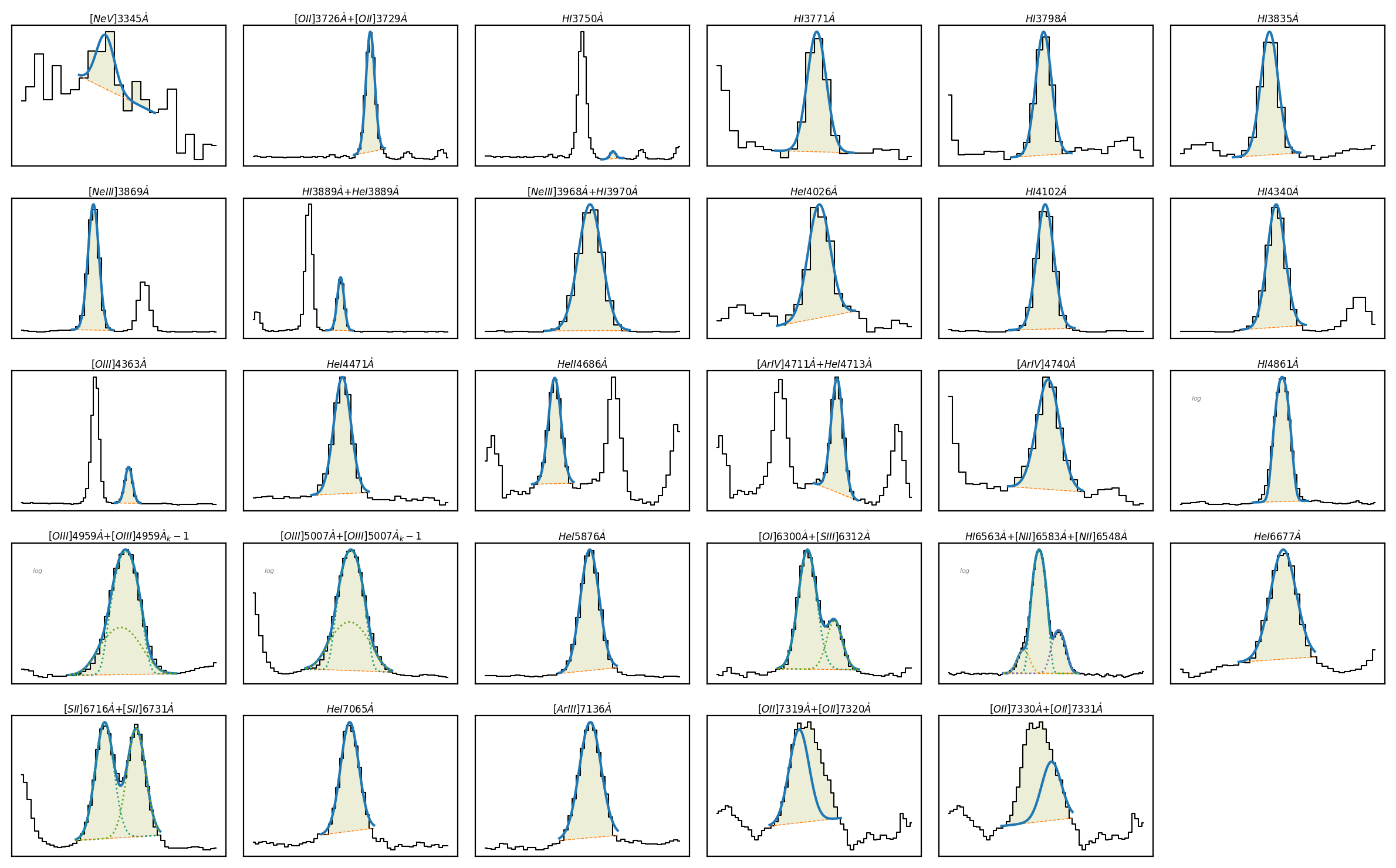
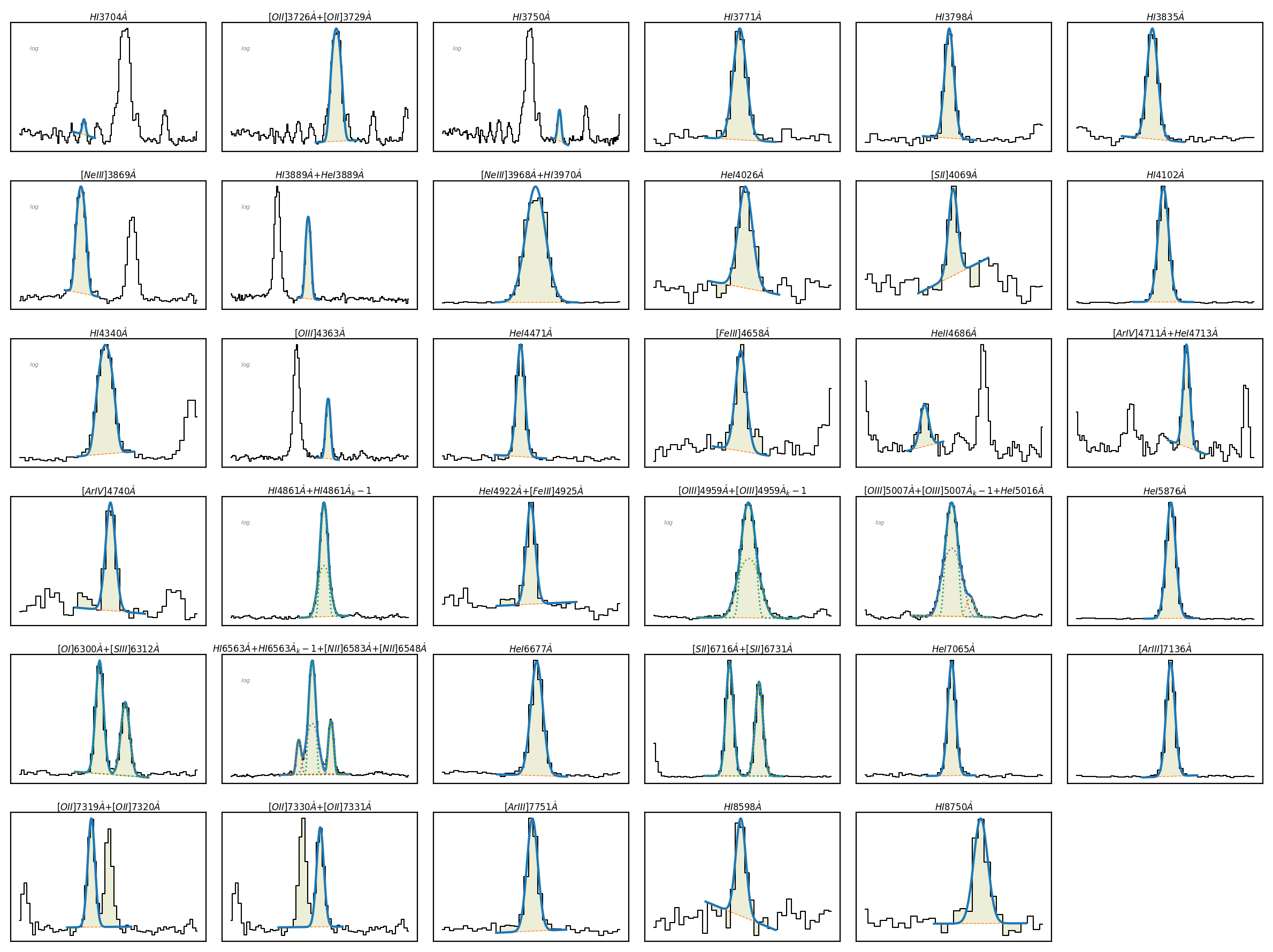
The fitted profiles can be checked with the \(\tt{lime.Spectrum.plot.grid}\) function:
gp_spec.plot.grid()

Behind the scenes, the \(\tt{lime.Spectrum.fit.frame}\) function performs multiple tasks:
When
line_detection=True, it runs the continuum fitting and peak detection algorithms described in the previous tutorials. The arguments for these functions are read from the inputfit_cfg. The progress bar will display the message (continuum fitting) (line detection) if these processes are active.The fitting configuration from the
default_line_fittingsection is updated with the entries fromgp121903_osiris_line_fitting:
Multi-level configuration files:#
If we look at the input defaulft line fitting configuration:
import pprint
pprint.pprint(obs_cfg['default_line_fitting'])
{'Ar4_4711A_m': 'Ar4_4711A+He1_4713A',
 'Fe3_4925A_m': 'He1_4922A+Fe3_4925A',
 'H1_3889A_m': 'H1_3889A+He1_3889A',
 'H1_6563A_b': 'H1_6563A+N2_6583A+N2_6548A',
 'H1_6563A_m': 'H1_6563A+N2_6583A+N2_6548A',
 'N1_5198A_m': 'N1_5198A+N1_5200A',
 'Ne3_3968A_m': 'Ne3_3968A+H1_3970A',
 'O1_6300A_b': 'O1_6300A+S3_6312A',
 'O2_3726A_b': 'O2_3726A+O2_3729A',
 'O2_3726A_m': 'O2_3726A+O2_3729A',
 'O2_7319A_m': 'O2_7319A+O2_7320A',
 'O2_7325A_b': 'O2_7319A_m+O2_7330A_m',
 'O2_7325A_m': 'O2_7319A_m+O2_7330A_m',
 'O2_7330A_m': 'O2_7330A+O2_7331A',
 'O3_5007A_b': 'O3_4959A+O3_5007A',
 'O3_5007A_m': 'O3_4959A+O3_5007A',
 'S2_6716A_b': 'S2_6716A+S2_6731A',
 'S2_6716A_m': 'S2_6716A+S2_6731A',
 'continuum': {'degree_list': [3, 6, 6], 'emis_threshold': [3, 2, 1.5]},
 'peaks_troughs': {'sigma_threshold': 3},
 'transitions': {'O2_3726A_m': {'wavelength': 3728.484},
                 'O2_7325A_b': {'wavelength': 7325.0},
                 'O2_7325A_m': {'wavelength': 7325.0}}}
and the object line fitting configuration:
pprint.pprint(obs_cfg['gp121903_osiris_line_fitting'])
{'H1_6563A_b': 'H1_6563A+N2_6583A+N2_6548A',
 'N2_6548A_amp': {'expr': 'N2_6583A_amp/2.94'},
 'N2_6548A_kinem': 'N2_6583A',
 'O2_7330A_m_kinem': 'O2_7319A_m',
 'O3_4959A_b': 'O3_4959A+O3_4959A_k-1',
 'O3_4959A_k-1_amp': {'expr': '<100.0*O3_4959A_amp', 'min': 0.0},
 'O3_4959A_k-1_sigma': {'expr': '>2.0*O3_4959A_sigma'},
 'O3_5007A_b': 'O3_5007A+O3_5007A_k-1',
 'O3_5007A_k-1_amp': {'expr': '<100.0*O3_5007A_amp', 'min': 0.0},
 'O3_5007A_k-1_sigma': {'expr': '>2.0*O3_5007A_sigma'},
 'S2_6716A_b': 'S2_6716A+S2_6731A',
 'S2_6731A_kinem': 'S2_6716A',
 'grouped_lines': ['O3_5007A_b', 'O3_4959A_b'],
 'map_band_vsigma': {'H1_4861A': 200,
                     'H1_6563A': 200,
                     'N2_6548A': 200,
                     'N2_6583A': 200,
                     'O3_4959A': 250,
                     'O3_5007A': 250},
 'rejected_lines': ['H1_3722A',
                    'H1_3734A',
                    'Fe3_4008A',
                    'S2_4076A',
                    'Fe2_4358A',
                    'Fe3_4881A',
                    'Fe3_4881A',
                    'Fe3_4986A',
                    'He1_5016A',
                    'Ar3_5192A',
                    'H1_8392A',
                    'H1_8413A',
                    'H1_8438A',
                    'H1_8467A',
                    'H1_8502A',
                    'H1_8545A']}
we notice the following differences:
The defaulft line fitting section includes the components for the composite lines, the parameters for the continuum fitting and peak_troughs thresholding and the wavelength definition for some merged lines.
The object line fitting also includes components for a few composite lines, the fitting parameter constrains for the blended profiles, and the grouped and rejected line lists for the \(\texttt{lime.Spectrum.retrieve.lines\_frame}\).
In the default behaviour, when update_default=True, the default line fitting configuration entries are updated with the object line fitting entries. For example, in the previous fitting, this is what \(\mathrm{LiMe}\) sees:
input_cfg = obs_cfg['default_line_fitting'].copy()
input_cfg.update(obs_cfg['gp121903_osiris_line_fitting'])
pprint.pprint(input_cfg)
{'Ar4_4711A_m': 'Ar4_4711A+He1_4713A',
 'Fe3_4925A_m': 'He1_4922A+Fe3_4925A',
 'H1_3889A_m': 'H1_3889A+He1_3889A',
 'H1_6563A_b': 'H1_6563A+N2_6583A+N2_6548A',
 'H1_6563A_m': 'H1_6563A+N2_6583A+N2_6548A',
 'N1_5198A_m': 'N1_5198A+N1_5200A',
 'N2_6548A_amp': {'expr': 'N2_6583A_amp/2.94'},
 'N2_6548A_kinem': 'N2_6583A',
 'Ne3_3968A_m': 'Ne3_3968A+H1_3970A',
 'O1_6300A_b': 'O1_6300A+S3_6312A',
 'O2_3726A_b': 'O2_3726A+O2_3729A',
 'O2_3726A_m': 'O2_3726A+O2_3729A',
 'O2_7319A_m': 'O2_7319A+O2_7320A',
 'O2_7325A_b': 'O2_7319A_m+O2_7330A_m',
 'O2_7325A_m': 'O2_7319A_m+O2_7330A_m',
 'O2_7330A_m': 'O2_7330A+O2_7331A',
 'O2_7330A_m_kinem': 'O2_7319A_m',
 'O3_4959A_b': 'O3_4959A+O3_4959A_k-1',
 'O3_4959A_k-1_amp': {'expr': '<100.0*O3_4959A_amp', 'min': 0.0},
 'O3_4959A_k-1_sigma': {'expr': '>2.0*O3_4959A_sigma'},
 'O3_5007A_b': 'O3_5007A+O3_5007A_k-1',
 'O3_5007A_k-1_amp': {'expr': '<100.0*O3_5007A_amp', 'min': 0.0},
 'O3_5007A_k-1_sigma': {'expr': '>2.0*O3_5007A_sigma'},
 'O3_5007A_m': 'O3_4959A+O3_5007A',
 'S2_6716A_b': 'S2_6716A+S2_6731A',
 'S2_6716A_m': 'S2_6716A+S2_6731A',
 'S2_6731A_kinem': 'S2_6716A',
 'continuum': {'degree_list': [3, 6, 6], 'emis_threshold': [3, 2, 1.5]},
 'grouped_lines': ['O3_5007A_b', 'O3_4959A_b'],
 'map_band_vsigma': {'H1_4861A': 200,
                     'H1_6563A': 200,
                     'N2_6548A': 200,
                     'N2_6583A': 200,
                     'O3_4959A': 250,
                     'O3_5007A': 250},
 'peaks_troughs': {'sigma_threshold': 3},
 'rejected_lines': ['H1_3722A',
                    'H1_3734A',
                    'Fe3_4008A',
                    'S2_4076A',
                    'Fe2_4358A',
                    'Fe3_4881A',
                    'Fe3_4881A',
                    'Fe3_4986A',
                    'He1_5016A',
                    'Ar3_5192A',
                    'H1_8392A',
                    'H1_8413A',
                    'H1_8438A',
                    'H1_8467A',
                    'H1_8502A',
                    'H1_8545A'],
 'transitions': {'O2_3726A_m': {'wavelength': 3728.484},
                 'O2_7325A_b': {'wavelength': 7325.0},
                 'O2_7325A_m': {'wavelength': 7325.0}}}
In this case, all the information has been combined, and the common entries (such as the O3_5007A_b definition) in the default line fitting are replaced by the object configuration.
Please note: If update_default=False, the algorithm will use the object line fitting configuration when available; otherwise, it will fall back to the default line fitting. For example, if we run:
gp_spec.clear_data()
gp_spec.fit.frame(bands=lineBandsFile, fit_cfg=obs_cfg, obj_cfg_prefix='gp121903_osiris', line_detection=True, update_default=False)
LiMe CRITICAL: Automatic line detection but the input configuration does not include a "continuum" entry with a "degree_list" and "emis_threshold" keys
LiMe WARNING: No "continuum" entry in input configuration file. No continuum fitting will be applied
LiMe WARNING: No "peaks_troughs" entry in input configuration file. No line thresholding will be applied
Line fitting progress (line detection):
[=         ] 10% of 38 lines (O2_3726A_m)
LiMe WARNING: The O2_3726A_m line has a "_m" suffix but its group lines components were not found on the input configuration file or lines database. It will be treated a single line
[== ] 26% of 38 lines (H1_3889A_m)
LiMe WARNING: The H1_3889A_m line has a "_m" suffix but its group lines components were not found on the input configuration file or lines database. It will be treated a single line
[== ] 28% of 38 lines (Ne3_3968A_m)
LiMe WARNING: The Ne3_3968A_m line has a "_m" suffix but its group lines components were not found on the input configuration file or lines database. It will be treated a single line
[===== ] 57% of 38 lines (Ar4_4711A_m)
LiMe WARNING: The Ar4_4711A_m line has a "_m" suffix but its group lines components were not found on the input configuration file or lines database. It will be treated a single line
[====== ] 65% of 38 lines (Fe3_4925A_m)
LiMe WARNING: The Fe3_4925A_m line has a "_m" suffix but its group lines components were not found on the input configuration file or lines database. It will be treated a single line
[======= ] 73% of 38 lines (N1_5198A_m)
LiMe WARNING: The N1_5198A_m line has a "_m" suffix but its group lines components were not found on the input configuration file or lines database. It will be treated a single line
[======== ] 81% of 38 lines (O1_6300A_b)
LiMe WARNING: The O1_6300A_b line has a "_b" suffix but its group lines components were not found on the input configuration file or lines database. It will be treated a single line
[========= ] 97% of 38 lines (O2_7325A_b)
LiMe WARNING: The O2_7325A_b line has a "_b" suffix but its group lines components were not found  on the input configuration file or lines database. It will be treated a single line
LiMe WARNING: Line O2_7325A was not found on the input bands database. It won't be measured
[==========] 100% of 38 lines (Ar3_7751A)
You can understand from the warnings that \(\mathrm{LiMe}\) did not find the components for some of lines, nor the continuum and peaks_troughs parameters, because those were only in the default_line_fitting. However for \(H\alpha\):
gp_spec.plot.bands('H1_6563A')
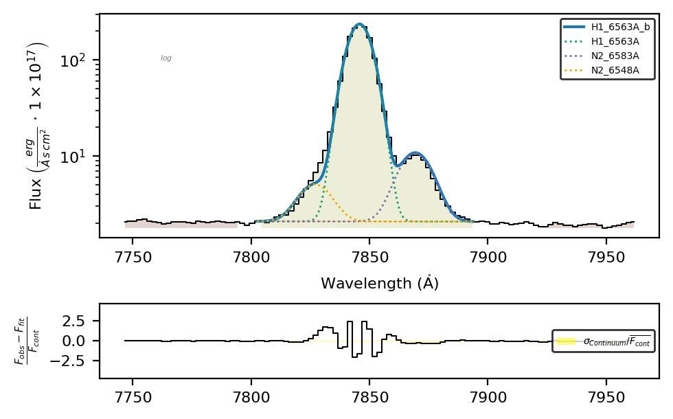
All the components are fitted because those were available the gp121903_osiris_line_fitting section.
Multiple-spectra fitting#
By combining the multi-level fitting configuration, we can easily fit the lines from multiple spectra. The code below loops through the spectra in the resources folder, prepares a lines frame for each object using the configuration data, and finally runs the continuum fitting, line thresholding, and line fitting with the \(\tt{lime.Spectrum.fit.frame}\) function.
# Instrument - file dictionary
files_dict = {'osiris': 'gp121903_osiris.fits', 'isis': 'IZW18_isis.fits',
'nirspec':'hlsp_ceers_jwst_nirspec_nirspec10-001027_comb-mgrat_v0.7_x1d-masked.fits', 'sdss':'SHOC579_SDSS_dr18.fits'}
# Instrument - object dictionary
object_dict = {'osiris':'gp121903', 'nirspec':'ceers1027', 'isis':'Izw18', 'sdss':'SHOC579'}
# Loop through the observations
for i, items in enumerate(object_dict.items()):
inst, obj = items
file_path = f'{data_folder}/{files_dict[inst]}'
redshift = obs_cfg[inst][obj]['z']
print('\n', obj, inst, redshift)
# Create the observation object
spec = lime.Spectrum.from_file(file_path, inst, redshift=redshift)
# Unit conversion for NIRSPEC object
if spec.units_wave != 'AA':
spec.unit_conversion('AA', 'FLAM')
# Revised bands for every object
bands_df = spec.retrieve.lines_frame(band_vsigma = 100, map_band_vsigma = {'O2_3726A': 200, 'O2_3729A': 200,
'H1_4861A': 200, 'H1_6563A': 200,
'N2_6548A': 200, 'N2_6583A': 200,
'O3_4959A': 250, 'O3_5007A': 250},
fit_cfg=obs_cfg, obj_cfg_prefix=f'{obj}_{inst}',
automatic_grouping=True, ref_bands=osiris_gp_df_path)
# Fit the lines via continuum fitting and line thresholding.
spec.fit.frame(bands_df, fit_cfg=obs_cfg, obj_cfg_prefix=f'{obj}_{inst}', line_detection=True)
# Save the measurements
spec.save_frame(f'../0_resources/results/{obj}_{inst}_line_frame.txt')
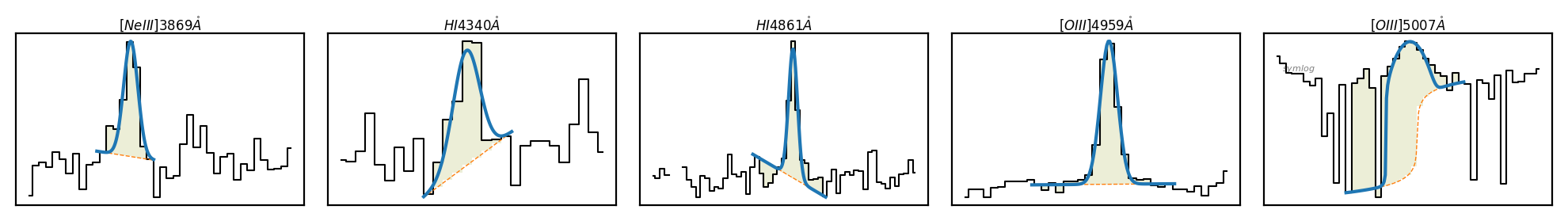
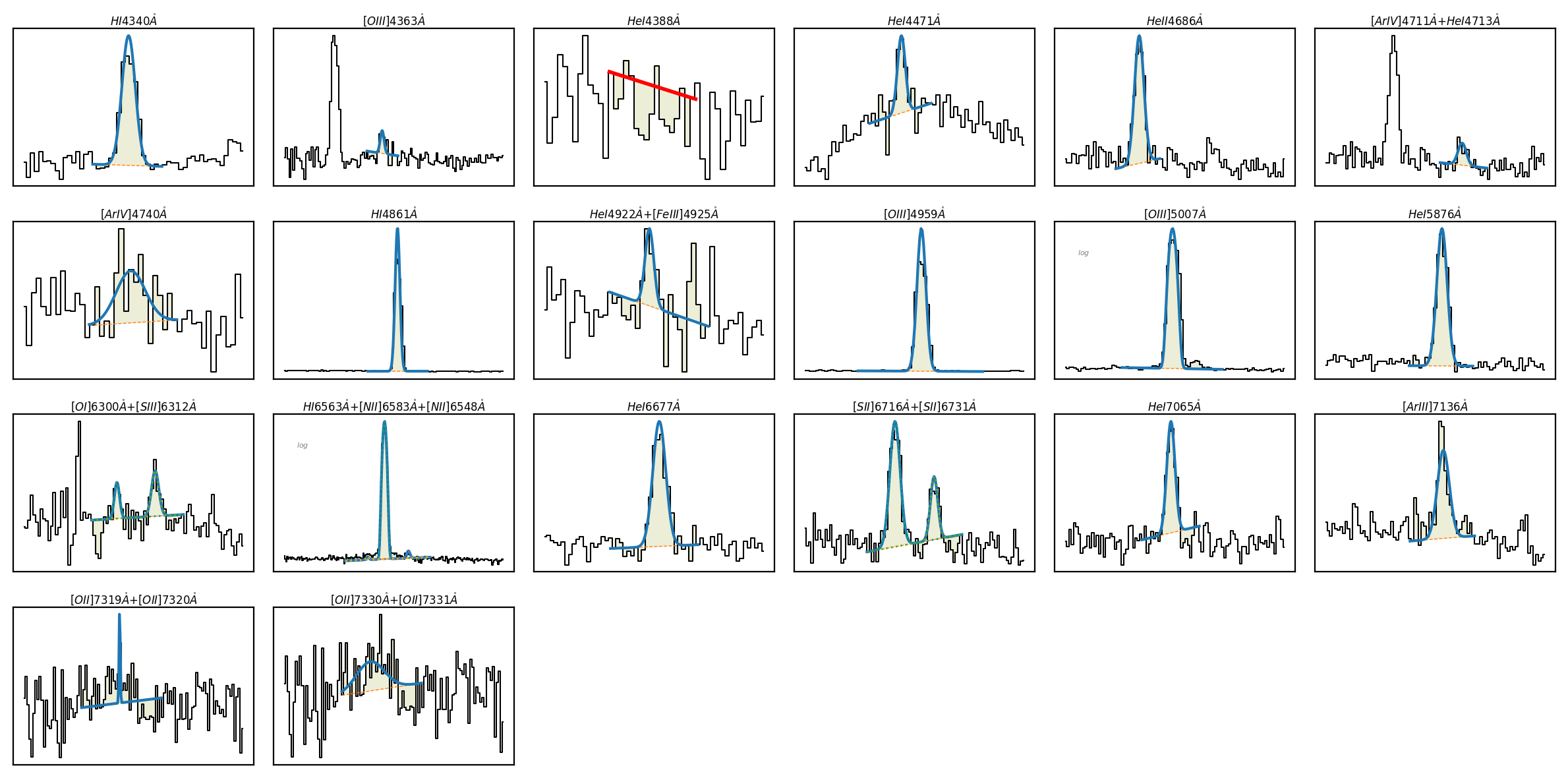
# Plot the profiles.plot.grid()
spec.plot.grid()
LiMe INFO: The observation does not include a normalization but the mean flux value is below 0.001. The flux will be automatically normalized by 1.000000045813705e-18.
 gp121903 osiris 0.19531

Line fitting progress (continuum fitting) (line detection):
[==========] 100% of 28 lines (O2_7325A_b)
LiMe INFO: The observation does not include a normalization but the mean flux value is below 0.001. The flux will be automatically normalized by 1e-08.
LiMe INFO: The observation does not include a normalization but the mean flux value is below 0.001. The flux will be automatically normalized by 1e-21.
 ceers1027 nirspec 7.8189

Line fitting progress (continuum fitting) (line detection):
[==========] 100% of 5 lines (O3_5007A)
LiMe INFO: The observation does not include a normalization but the mean flux value is below 0.001. The flux will be automatically normalized by 9.99999983775159e-18.
 Izw18 isis 0.0026

Line fitting progress (continuum fitting) (line detection):
[=         ] 15% of 19 lines (He1_4388A)
LiMe WARNING: Gaussian fit uncertainty estimation failed for He1_4388A
[==========] 100% of 19 lines (O2_7325A_b)
LiMe WARNING: Line H1_3721A was not found on the database
 SHOC579 sdss 0.0475

Line fitting progress (continuum fitting) (line detection):
[==        ] 23% of 34 lines (H1_3889A_m)
/home/vital/anaconda3/envs/lime2/lib/python3.12/site-packages/lmfit/models.py:320: RankWarning: Polyfit may be poorly conditioned
  out = np.polyfit(x, data, self.poly_degree)
/home/vital/anaconda3/envs/lime2/lib/python3.12/site-packages/lmfit/models.py:320: RankWarning: Polyfit may be poorly conditioned
  out = np.polyfit(x, data, self.poly_degree)
[==========] 100% of 34 lines (H1_8750A)))
Takeaways#
To measure multiple lines in a spectrum, you can use the \(\tt{lime.Spectrum.fit.frame}\) function.
The first input (
bands) is a lines frame containing the lines you want to fit.By setting
line_detection=True, the function will run the continuum fitting and line thresholding using the parameters infit_cfg.
The second input (
fit_cfg) is a configuration dictionary or file containing the parameters for the fitting process.This function supports two configuration levels: a default configuration that serves as a baseline, and an object configuration for individual observations. You can specify the parameter sections for each configuration layer using the
default_cfg_prefixandobj_cfg_prefixarguments.By default, the object line fitting updates the default line fitting. This minimizes the amount of writing needed in your configuration file. However, you can set
update_default=Falseso that the object configuration is used as is, or falls back to the default configuration.You can read the function documentation in the API.