Loading observations#
As it was mention in the introduction to observations \(\mathrm{LiMe}\) can create observations directly from some instrument .fits files:
import numpy as np
from astropy.io import fits
from pathlib import Path
from astropy.wcs import WCS
import lime
import astropy

# Specifying 2_guides:
data_folder = Path('../0_resources/spectra')
sloan_SHOC579 = data_folder/'sdss_dr18_0358-51818-0504.fits'

# Create the observation
shoc579 = lime.Spectrum.from_file(sloan_SHOC579, instrument='sdss', redshift=0.0475)

# Plot the spectrum
shoc579.plot.spectrum(rest_frame=True)
The complete list of supported and their configuration can be access running the \(\tt{lime.show\_instrument\_cfg()}\) command:
lime.show_instrument_cfg()
Long-slit ".fits" observation instrument configuration:
 0	nirspec        	units_wave: um        	units_flux: Jy        	pixel_mask: nan     	res_power: None
 1	nirspec_grizli 	units_wave: um        	units_flux: uJy       	pixel_mask: nan     	res_power: None
 2	isis           	units_wave: Angstrom  	units_flux: FLAM      	pixel_mask: nan     	res_power: None
 3	osiris         	units_wave: Angstrom  	units_flux: FLAM      	pixel_mask: nan     	res_power: None
 4	cos            	units_wave: Angstrom  	units_flux: FLAM      	pixel_mask: nan     	res_power: None
 5	sdss           	units_wave: Angstrom  	units_flux: 1e-17*FLAM	pixel_mask: nan     	res_power: None
 6	desi           	units_wave: Angstrom  	units_flux: 1e-17*FLAM	pixel_mask: nan     	res_power: None
 7	text           	units_wave: Angstrom  	units_flux: FLAM      	pixel_mask: None    	res_power: None

Cube ".fits" observation instrument configuration:
 0	manga          	units_wave: Angstrom  	units_flux: 1e-17*FLAM	pixel_mask: nan     	res_power: None
 1	muse           	units_wave: Angstrom  	units_flux: 1e-20*FLAM	pixel_mask: nan     	res_power: None
 2	megara         	units_wave: Angstrom  	units_flux: Jy        	pixel_mask: nan     	res_power: None
 3	miri           	units_wave: um        	units_flux: MJy       	pixel_mask: nan     	res_power: None
 4	kcwi           	units_wave: AA        	units_flux: 1e16*FLAM 	pixel_mask: nan     	res_power: None
However, if your instrument .fits file is not supported, you can still create the observations by providing the spectroscopic data. In this guide we are going to show some examples.
Please remember: The reader is recomended to check the official .fits documentation from astropy to familiarize with this format.
a) Osiris long-slit#
In the sample examples/sample_data you have the spectrum from the OSIRIS instrument at the GTC (Gran Telescopio de Canarias). This file contains the flux array but you must reconstruct the wavelength array from the header CRVAL1, CD1_1 and NAXIS1 keys:
# Spectrum address
fits_path = data_folder/'gp121903_osiris.fits'

# Data extension index
extension = 0

# Open the fits file
with fits.open(fits_path) as hdul:
    flux_array, header = hdul[extension].data, hdul[extension].header
In the code above, we use the with context manager. This structure makes sure that the file is closed once we extract the data. This is a safe practice in the case of large .fits files.
Now, we are going to compute the wavelength array:
#Lowest wavelength value
w_min = header['CRVAL1']

# Resolution in angstroms per pixel
dw = header['CD1_1']

# Number of pixels
n_pixels = header['NAXIS1']

# Array computation
w_max = w_min + dw * n_pixels
wave_array = np.linspace(w_min, w_max, n_pixels, endpoint=False)
print(wave_array)
[ 3626.97753906  3629.04561139  3631.11368372 ... 10236.5367069
 10238.60477923 10240.67285156]
The units on the spectrum arrays should also be specified on the .fits header:
print(f'Wavelength array: {header["WAT1_001"]}')
print(f'Flux array: {header["BUNIT"]}')
Wavelength array: wtype=linear label=Wavelength units=Angstroms
Flux array: erg/cm2/s/A
Now, we are going to create the \(\tt{lime.Spectrum}\) from the raw data. This object has the following arguments:
redshift: Object redshift
norm_flux Flux normalization
units_wave: Spectrum wavelength units. The default values is Angstroms.
units_flux: Spectrum flux units. The default value is FLAM \(\mathrm{\left(\frac{\text{erg}}{\text{s} \cdot \text{cm}^2 \cdot \mathring{A}}\right)}\)
pixel_mask: Indeces to mask or entries to mask on the wavelength, flux and uncertainty arrays.
res_power: Observation resolving power.
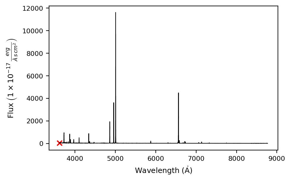
obj = lime.Spectrum(wave_array, flux_array, redshift=0.19531)
obj.plot.spectrum(rest_frame=True)
LiMe INFO: The observation does not include a normalization but the mean flux value is below 0.001. The flux will be automatically normalized by 1.000000045813705e-18.
In the observation above, we did not introduce a flux normalization but \(\mathrm{LiMe}\) calculated one for us.
b) Sloan long-slit#
\(\mathrm{LiMe}\) can read .fits files from the SDSS survey survey as we saw above, but let’s check this optional method:
# Open the fits file
extension = 1
with fits.open(sloan_SHOC579) as hdul:
    data = hdul[extension].data
    header = hdul[extension].header
The flux key indexes the flux. This value is normalized by so we are going to define the units including this scale:
flux_array = data['flux']
units_flux = '1e-17*FLAM'
The flux uncertainty is stored as the inversed of the variance. The bad values in this array are set to zero, hence, we are going to mask these values to compute the error spectrum.
ivar_array = data['ivar']
err_array = np.sqrt(1/ivar_array)
pixel_mask = ivar_array == 0
/tmp/ipykernel_158862/3510536718.py:2: RuntimeWarning: divide by zero encountered in divide
  err_array = np.sqrt(1/ivar_array)
Finally, the wavelength array is stored in logarithmic scale and they are accessed via the loglam key:
wave_vac_array = np.power(10, data['loglam'])
Now we can create the Spectrum object:
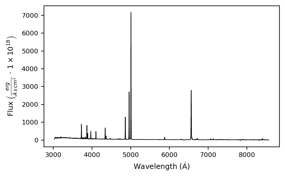
obj = lime.Spectrum(wave_vac_array, flux_array, err_array, pixel_mask=pixel_mask, units_flux=units_flux, redshift=0.0475)
obj.plot.spectrum(rest_frame=True)
If you don’t not provide a pixel mask, \(\mathrm{LiMe}\) will try to mask non-physical entries:
obj = lime.Spectrum(wave_vac_array, flux_array, err_array, units_flux=units_flux, redshift=0.0475)
obj.plot.spectrum(rest_frame=True)
LiMe INFO: The input err_flux array contains "inf" entries a pixel_mask will be generated automatically
Please remember: The reader is adviced to define their own pixel mask, even if \(\mathrm{LiMe}\) will check for np.nan and np.inf entries
c) MANGA IFU cube#
Now, we are going to open the MANGA integrated field unit observation of SHOC579:
fits_path = data_folder/'manga-8626-12704-LOGCUBE.fits.gz'
This file is compressed, however, the astropy.io.fits.open can read it. However, keep in mind that reading compressed files takes more time:
# Open the MANGA cube fits file
with fits.open(fits_path) as hdul:

    # Wavelength 1D array
    wave = hdul['WAVE'].data

    # Flux 3D array
    flux_cube = hdul['FLUX'].data
    units_flux = '1e-17*FLAM'

    # Convert inverse variance cube to standard error, masking 0-value pixels first
    ivar_cube = hdul['IVAR'].data
    err_cube = np.sqrt(1/ivar_cube)
    pixel_mask_cube = ivar_cube == 0

    # Header
    hdr = hdul['FLUX'].header
/tmp/ipykernel_158862/2371804064.py:13: RuntimeWarning: divide by zero encountered in divide
  err_cube = np.sqrt(1/ivar_cube)
The header of .fits spectra usually contains the astronomical coordinates of the observation. \(\mathrm{LiMe}\) relies on World Coordidnate System to plot the IFU data and export the coordinates to the output .fits files with your measurements. You can create the WCS object from the corresponding .fits header:
# WCS from the observation
wcs = WCS(hdr)
WARNING: FITSFixedWarning: PLATEID = 8626 / Current plate
a string value was expected. [astropy.wcs.wcs]
WARNING: FITSFixedWarning: 'datfix' made the change 'Set MJD-OBS to 57277.000000 from DATE-OBS'. [astropy.wcs.wcs]
Now, we have all the create our Cube object:
cube = lime.Cube(wave, flux_cube, err_cube, redshift=0.0475, units_flux=units_flux, pixel_mask=pixel_mask_cube)
Now you can extract individual spaxels to analyse the object lines. Each spaxel will have its corresponding error spectrum and pixel mask
# Extract spaxel
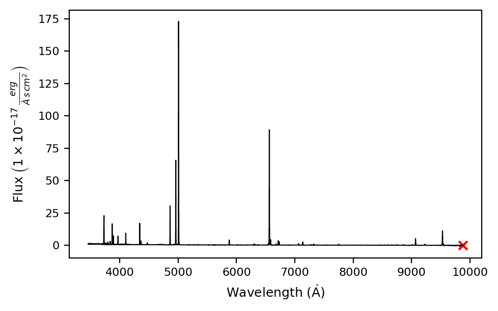
spaxel = cube.get_spectrum(38, 35)
# Plot spectrum
spaxel.plot.spectrum(rest_frame=True)
Takeaways#
\(\mathrm{LiMe}\) can create observations directly from some .fits files for some instruments. Otherwise you can always create \(\tt{lime.Spectrum}\) or \(\tt{lime.Cube}\) objects directly from the scientific data.
\(\mathrm{LiMe}\) will compute a pixel mask for non physical entries and compute a flux normalization if the user does not provide them. However, the user is recomended to provide his/her own.