Measurements description

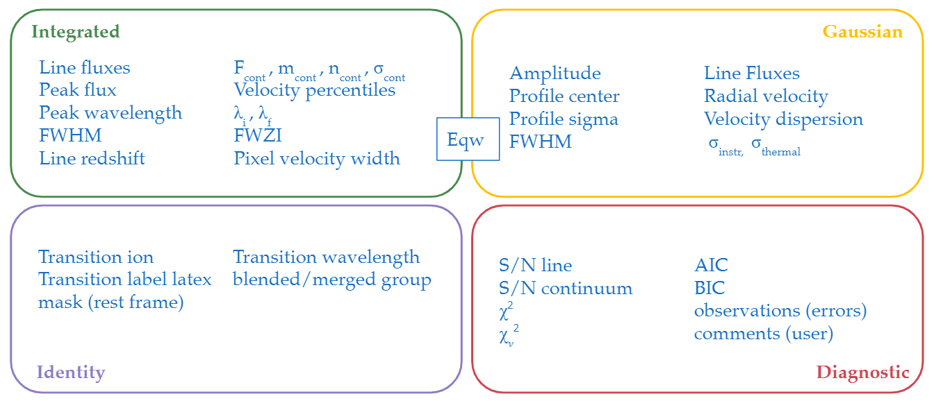
This section describes the parameters measured by \(\mathrm{LiMe}\). Unless otherwise noted, these parameters have the same notation in the output measurements log as in the lime.Spectrum.frame dataframe column headers.

Identification

These parameters are part of the inputs provided by the user to label the line analysis:

• line (.line, str): The name of the line the measurements belong to. It follows the \(\mathrm{LiMe}\) line notation format.

• band (.band, np.array()): A six-value vector with the line band wavelength limits. In the lime.Spectrum object, the mask is stored as a vector under the lime.Spectrum.mask attribute. In the .log, the wavelengths are stored in individual columns with the headers: w1, w2, w3, w4, w5 and w6.

• group_label (.group_label, str): The labels of all components in a blended line, joined by +. For single lines this parameter is None. For example, a blended H\(\alpha\)-[NII] complex would appear as:

    H1_6563A+N2_6584A+N2_6548A
  

• wavelength: The theoretical, rest-frame wavelength of the emission line. If the line is not found on the \(\mathrm{LiMe}\) database, it is derived from the .line label. By default, the transition is in air values for transitions between 2000-10000 angstroms.

• particle: The particle responsible for the line photons. This value is derived from the line label provided by the user.

• latex_label: The transition classical notation in LaTeX format. This string includes the profile components if they were provided during the fitting.

• shape (.shape, str): Whether the line is observed in emission or absorption. The two possible values are emi for emission lines and abs for absorption lines.

• profile (.profile, str): The functional form used to fit the line profile: g (Gaussian), l (Lorentzian), v (Voigt), pv (Pseudo-Voigt), pp (Pseudo-Power law), p (Broken Power law), or e (Exponential).

• pixel_mask (.pixel_mask, str): A string specifying the pixel intervals excluded from the line fitting, as provided by the user in the fitting configuration. For single lines with no masked pixels this parameter is none.

Integrated properties

These measurements are independent of the line profile:

Attention

In the output measurements log and the lime.Spectrum.frame, these parameters have the same flux units as the input spectrum. However, the attributes of the lime.Spectrum object are normalized by the .norm_flux constant provided by the user at the lime.Spectrum definition.

• peak_wave (.peak_wave, float): The wavelength of the most intense pixel value (or lowest for an absorption) in the line region.

• peak_flux (.peak_flux, float): The flux of the highest pixel value (or lowest for an absorption) in the line region.

• m_cont (.m_cont, float): The gradient of a linear continuum fitted to the adjacent continuum bands:

  \[y = m \cdot x + n\]

  The fitting method depends on the cont_source parameter. For the adjacent method, scipy.curve_fit is used on both adjacent bands (w1–w2 and w5–w6) with absolute_sigma=True. For the central method, a two-point fit is computed analytically from the edges of the line band (w3 and w4).

• m_cont_err (.m_cont_err, float): The uncertainty on the continuum slope .m_cont, propagated from the scipy.curve_fit covariance matrix for the adjacent method or analytically from the anchor pixel errors for the central method.

• n_cont (.n_cont, float): The intercept of the linear continuum fit described above.

• n_cont_err (.n_cont_err, float): The uncertainty on the continuum intercept .n_cont, propagated analogously to .m_cont_err.

• cont (.cont, float): The flux of the linear continuum evaluated at .peak_wave.

• cont_err (.cont_err, float): The uncertainty on the continuum at .peak_wave. For the adjacent method (via scipy.curve_fit), this is propagated from the correlated slope and intercept uncertainties including the covariance term \(\mathrm{Cov}(m, n)\). For the central method (two-point fit), this is propagated analytically from the independent anchor pixel errors \(e_0\) and \(e_N\):

  \[\sigma_{cont} = \sqrt{\left(\frac{x_N - x_{peak}}{\Delta x}\,e_0\right)^2 + \left(\frac{x_{peak} - x_0}{\Delta x}\,e_N\right)^2}\]

  where \(\Delta x = x_N - x_0\) and \(x_{peak}\) is .peak_wave.

• intg_flux (.intg_flux, float): The integrated flux of the emission line. This value is calculated via a Monte Carlo algorithm:

  1. If the pixel error spectrum is not provided by the user, the algorithm uses the line .cont_err as a uniform uncertainty for all the line pixels.

  2. The pixel error is added stochastically to each pixel in the line region mask.

  3. The flux in the line region is summed, taking into consideration the line region averaged pixel width and removing the contribution of the linear continuum.

  4. Steps 2–3 are repeated 1000 times. The mean flux value from the resulting array is taken as the integrated flux.

• intg_err (.intg_err, float): The integrated flux uncertainty, derived from the standard deviation of the Monte Carlo flux calculation described above.

  Attention

  Blended line components share the same .intg_flux and .intg_err values.

• eqw (.eqw, float or np.array()): The equivalent width of the emission line, calculated from:

  \[Eqw = \int_{\lambda_1}^{\lambda_2}\frac{F_c - F_\lambda}{F_c}\,d\lambda = \int_{\lambda_1}^{\lambda_2}\frac{F_{line}}{F_c}\,d\lambda\]

  where \(F_c\) is the flux of the linear continuum at the peak wavelength (.cont) and \(F_\lambda\) is the spectrum flux. In single lines, \(F_{line}\) is the integrated flux (.intg_flux); in blended lines, the corresponding Gaussian flux (.profile_flux) is used. The integration limits are w3 and w4 from the user mask.

• eqw_err (.eqw_err, float or np.array()): The uncertainty on the equivalent width, propagated via Monte Carlo from the continuum flux (.cont, .cont_err) and the line flux uncertainty.

• z_line (.z_line, float): The emission line redshift:

  \[z_{\lambda} = \frac{\lambda_{obs}}{\lambda_{theo}} - 1\]

  where \(\lambda_{obs}\) is .peak_wave. In blended lines, this variable is computed using the same .peak_wave for all transitions (the most intense pixel in the line band).

• FWHM_i (.FWHM_i, float): The Full Width at Half Maximum in \(\mathrm{km/s}\) computed from the integrated profile. The algorithm identifies the pixels above half the line peak flux and subtracts the blue edge velocity from the red edge velocity.

  Attention

  This measurement is only available for lines whose width spans more than 15 pixels.

• snr_line (.snr_line, float): The signal-to-noise ratio of the emission line, following the definition by Rola et al. 1994:

  \[\frac{S}{N}_{line} \approx \frac{\sqrt{2\pi}}{6}\frac{A_{line}}{\sigma_{cont}}\sqrt{N} \approx \frac{F_{line}}{\sigma_{cont}\cdot\sqrt{N}}\]

  where \(A_{line}\) is the line amplitude, \(F_{line}\) is the integrated flux (.intg_flux), \(\sigma_{cont}\) is the continuum flux standard deviation (.cont_err), and \(N\) is the number of pixels in the input line band. In single lines, \(N \approx 6\sigma\) where \(\sigma\) is the Gaussian profile standard deviation.

• snr_cont (.snr_cont, float): The signal-to-noise ratio of the continuum in the line region:

  \[\frac{S}{N}_{cont} = \frac{F_{cont}}{\sigma_{cont}}\]

  where \(F_{cont}\) is the continuum flux at the peak wavelength (.cont) and \(\sigma_{cont}\) is the continuum flux standard deviation (.cont_err).

• v_med (.v_med, float): The median velocity of the emission line. The emission line wavelength array is converted to velocity units using:

  \[V\,(\mathrm{km/s}) = c \cdot \left(\frac{\lambda_{obs}}{\lambda_{peak}} - 1\right)\]

  where \(c = 299792.458\,\mathrm{km/s}\), \(\lambda_{obs}\) is the wavelength array between w3 and w4, and \(\lambda_{peak}\) is .peak_wave.

• v_50 (.v_50, float): The velocity corresponding to the 50th percentile of the emission line flux distribution. A cumulative sum of the line flux array is computed, multiplied by .pixelWidth, and divided by .intg_flux to obtain the fractional flux at each pixel between w3 and w4. This fractional flux vector is then interpolated against the velocity array described above.

  Attention

  This measurement is only available for lines whose width spans more than 15 pixels.

• v_5 (.v_5, float): The velocity at the 5th percentile of the emission line flux. See .v_50 for the calculation procedure.

• v_10 (.v_10, float): The velocity at the 10th percentile of the emission line flux. See .v_50 for the calculation procedure.

• v_90 (.v_90, float): The velocity at the 90th percentile of the emission line flux. See .v_50 for the calculation procedure.

• v_95 (.v_95, float): The velocity at the 95th percentile of the emission line flux. See .v_50 for the calculation procedure.

• sigma_thermal (.sigma_thermal, np.array()): The thermal broadening contribution to the line width in \(\mathrm{km/s}\), computed from the kinetic theory of gases:

  \[\sigma_{th} = \frac{1}{1000}\sqrt{\frac{k_B\,T}{m}}\]

  where \(k_B\) is the Boltzmann constant, \(T\) is the gas temperature in Kelvin, and \(m\) is the atomic mass of the ion responsible for the transition. One value is computed per profile component since different ions have different atomic masses.

• sigma_instr (.sigma_instr, float): The instrumental broadening contribution to the line width in \(\mathrm{km/s}\), derived from the spectral resolving power \(R = \lambda / \Delta\lambda\):

  \[\sigma_{instr} = \frac{\lambda}{R \cdot 2\sqrt{2\ln 2} \cdot 1000}\]

  where \(\bar{\lambda}\) is the mean wavelength of the line region and the \(2\sqrt{2\ln 2}\) factor converts from the instrumental FWHM to a Gaussian \(\sigma\). If \(R\) is provided as a scalar, a single value is computed from the mean wavelength; if \(R\) is an array, the mean is taken over the unmasked pixels in the line region. If no resolving power is provided, this parameter is NaN.

• FWZI (.FWZI, float): The Full Width at Zero Intensity in \(\mathrm{km/s}\). Computed as the velocity difference between the 1st and 99th percentile velocity points of the emission line flux distribution:

  \[FWZI = v_{99} - v_{1}\]

  using the same percentile velocity procedure described for .v_50.

Profile properties

These measurements are dependent on the model selected to fit the line profile. For example in the case of a Gaussian or multi-Gaussian profile:

\[F_{\lambda} = \sum_{i} A_i \, e^{-\frac{\left(\lambda - \mu_i\right)^2}{2\sigma_i}}\]

where \(F_\lambda\) is the Gaussian component profile flux. \(A_i\) is the amplitude of a Gaussian component measured with respect to the linear continuum (.cont), \(\mu_i\) is the component centre, and \(\sigma_i\) is the standard deviation. \(A_i\) carries the input flux units (lime.Spectrum.flux), while \(\mu_i\) and \(\sigma_i\) carry the input wavelength units (lime.Spectrum.wave).

• amp (.amp, np.array()): The amplitude of the Gaussian profiles, in the input flux units (lime.Spectrum.flux).

• amp_err (.amp_err, np.array()): The uncertainty on the Gaussian profile amplitudes, in the input flux units.

• center (.center, np.array()): The central wavelength of each Gaussian component, in the input wavelength units (lime.Spectrum.wave).

• center_err (.center_err, np.array()): The uncertainty on the Gaussian component central wavelengths.

• sigma (.sigma, np.array()): The standard deviation of each Gaussian component, in the input wavelength units.

• sigma_err (.sigma_err, np.array()): The uncertainty on the Gaussian component standard deviations.

• v_r (.v_r, np.array()): The radial velocity of each Gaussian component in \(\mathrm{km/s}\):

  \[v_{r} = c \cdot \left(\frac{\lambda_{center}}{\lambda_{ref}} - 1\right)\]

  where \(c = 299792.458\,\mathrm{km/s}\), \(\lambda_{center}\) is the Gaussian central wavelength (.center), and \(\lambda_{ref}\) is the reference wavelength. In non-blended lines, \(\lambda_{ref}\) is the observed peak wavelength (.peak_wave). In blended lines, \(\lambda_{ref}\) is the component transition wavelength (.wave) shifted to the observed frame using the redshift provided by the user at lime.Spectrum.

• v_r_err (.v_r_err, np.array()): The uncertainty on the Gaussian component radial velocities in \(\mathrm{km/s}\).

• sigma_vel (.sigma_vel, np.array()): The Gaussian component standard deviation in \(\mathrm{km/s}\):

  \[\sigma_{v}\,(\mathrm{km/s}) = c \cdot \frac{\sigma}{\lambda_{ref}}\]

  where \(c = 299792.458\,\mathrm{km/s}\), \(\sigma\) is the Gaussian profile standard deviation (.sigma), and \(\lambda_{ref}\) is the reference wavelength (see .v_r for the blended vs. non-blended distinction).

• sigma_vel_err (.sigma_vel_err, float or np.array()): The uncertainty on the Gaussian component standard deviations in \(\mathrm{km/s}\).

• gamma (.gamma, np.array()): The Lorentzian half-width at half-maximum of each Voigt profile component, in the input wavelength units (lime.Spectrum.wave). Only populated for Voigt (v) profiles.

• gamma_err (.gamma_err, np.array()): The uncertainty on the Lorentzian half-width parameter, in the input wavelength units.

• frac (.frac, np.array()): The mixing fraction \(\eta_i \in [0, 1]\) of each pseudo-Voigt (pv) or pseudo-power (pp) profile component. A value of 1 corresponds to a pure Lorentzian and 0 to a pure Gaussian.

• frac_err (.frac_err, np.array()): The uncertainty on the mixing fraction parameter.

• alpha (.alpha, np.array()): The exponential decay parameter \(\alpha_i\) of each exponential (e) profile component, in the inverse of the input wavelength units. Controls the rate of decay as \(e^{-\alpha_i|x - \mu_i|}\).

• alpha_err (.alpha_err, np.array()): The uncertainty on the exponential decay parameter.

• a (.a, np.array()): The normalisation parameter of each broken power law (p) profile component.

• a_err (.a_err, np.array()): The uncertainty on the normalisation parameter.

• b (.b, np.array()): The blue-side power law index of each broken power law (p) profile component, in the input wavelength units.

• b_err (.b_err, np.array()): The uncertainty on the blue-side power law index.

• c (.c, np.array()): The red-side power law index of each broken power law (p) profile component, in the input wavelength units.

• c_err (.c_err, np.array()): The uncertainty on the red-side power law index.

• profile_flux (.profile_flux, np.array()): The flux of each line profile component, obtained by integrating the profile model over wavelength. The formula depends on the profile type assigned to the component:

  Gaussian (g) — the integral \(\int_{-\infty}^{\infty} A\,e^{-(x-\mu)^2/2\sigma^2}\,dx\) is solved by substituting \(u = x - \mu\) to remove the centre, then \(t = u/(\sigma\sqrt{2})\) to reduce it to the standard Gaussian integral \(\int_{-\infty}^{\infty} e^{-t^2}\,dt = \sqrt{\pi}\). The substitution Jacobian contributes a factor of \(\sigma\sqrt{2}\), giving the exact result:

  \[F_{i} = \sqrt{2\pi} \cdot A_i \cdot \sigma_i\]

  Lorentzian (l) — the integral \(\int_{-\infty}^{\infty} \frac{A}{1+((x-\mu)/\sigma)^2}\,dx\) is solved by substituting \(u = (x-\mu)/\sigma\), reducing it to \(A\sigma\int_{-\infty}^{\infty}\frac{1}{1+u^2}\,du = A\sigma\pi\), giving the exact result:

  \[F_{i} = \pi \cdot A_i \cdot \sigma_i\]

  Pseudo-Voigt (pv) — the true Voigt profile is the convolution of a Gaussian and a Lorentzian and has no closed-form integral. Thompson, Cox & Hastings (1987) introduced the pseudo-Voigt as a practical linear mixture approximation \(V \approx \eta\,L + (1-\eta)\,G\), where \(\eta \in [0,1]\) is a mixing fraction (.frac). The area follows by linearity:

  \[F_{i} = \eta_i \cdot \pi \cdot A_i \cdot \sigma_i + (1 - \eta_i) \cdot \sqrt{2\pi} \cdot A_i \cdot \sigma_i\]

  Exponential (e) — the profile is defined as \(A\,e^{-\alpha|x-\mu|}\). Substituting \(u = x - \mu\) and exploiting symmetry, \(\int_{-\infty}^{\infty} e^{-\alpha|u|}\,du = 2\int_0^{\infty} e^{-\alpha u}\,du = 2/\alpha\), giving the exact result:

  \[F_{i} = \frac{2 A_i}{\alpha_i}\]

  where \(\alpha_i\) is the exponential decay parameter of the component (.alpha).

  Pseudo-power (pp) — uses the same linear mixture formula as the pseudo-Voigt with mixing fraction .frac:

  \[F_{i} = \eta_i \cdot \pi \cdot A_i \cdot \sigma_i + (1 - \eta_i) \cdot \sqrt{2\pi} \cdot A_i \cdot \sigma_i\]

  Power (p): not yet implemented; returns NaN.

  In all cases, \(A_i\) is the component amplitude (.amp) and \(\sigma_i\) is the standard deviation (.sigma). The flux and its uncertainty are computed via Monte Carlo sampling of the profile parameters, with the mean and standard deviation of the resulting distribution taken as .profile_flux and .profile_flux_err respectively.

• profile_flux_err (.profile_flux_err, np.array()): The uncertainty on the profile component fluxes. This is the standard deviation of the Monte Carlo flux distribution described above, where each realisation draws the profile parameters from their 1\(\sigma\) LmFit uncertainties.

  Note

  The independent sampling approximation ignores any covariance between profile parameters (e.g. between .amp and .sigma) reported by the LmFit covariance matrix.

• FWHM_p (.FWHM_p, np.array()): The Full Width at Half Maximum of each profile component in the input wavelength units. The formula depends on the profile type assigned to the component:

  Gaussian (g) — solved from \(e^{-(x/\sigma)^2/2} = 1/2\), giving \(x = \sigma\sqrt{2\ln 2}\) at each half-maximum point, and therefore:

  \[FWHM_g = 2\sqrt{2\ln 2}\,\sigma_i \approx 2.3548\,\sigma_i\]

  Lorentzian (l) — solved from \(\frac{1}{1+(x/\sigma)^2} = 1/2\), giving \(x = \sigma\) at each half-maximum point, and therefore:

  \[FWHM_l = 2\sigma_i\]

  Voigt (v) — the FWHM of the true Voigt profile has no closed form. The approximation of Thompson, Cox & Hastings (1987), accurate to better than 0.02%, is used:

  \[FWHM_v \approx 0.5346\,FWHM_l + \sqrt{0.2166\,FWHM_l^2 + FWHM_g^2}\]

  where \(FWHM_g\) and \(FWHM_l\) are the Gaussian and Lorentzian FWHMs defined above.

  Exponential (e) — solved from \(e^{-\alpha|x|} = 1/2\), giving \(|x| = \ln 2/\alpha\) at each half-maximum point, and therefore:

  \[FWHM_e = \frac{2\ln 2}{\alpha_i}\]

  where \(\alpha_i\) is the exponential decay parameter of the component (.alpha).

  Pseudo-Voigt (pv) and Pseudo-power (pp): not yet implemented; returns the Gaussian FWHM as a placeholder.

  Power (p): not yet implemented; returns NaN.

Diagnostics

These parameters provide qualitative or quantitative diagnostics on the line measurement.

• chisqr (.chisqr, float): The \(\chi^2\) statistic calculated by LmFit.

• redchi (.redchi, float): The reduced \(\chi^2\) statistic calculated by LmFit:

  \[\chi_{\nu}^2 = \frac{\chi^2}{N - N_{varys}}\]

  where \(\chi^2\) is divided by the number of data points \(N\) minus the number of free parameters \(N_{varys}\).

• aic (.aic, float): The Akaike information criterion calculated by LmFit.

• bic (.bic, float): The Bayesian information criterion calculated by LmFit.

• observations (.observations, str): Errors or warnings generated during the fitting of the line (not yet implemented).

• comments (.comments, str): Left empty for the user to store custom comments.