Continuum fitting

\(\mathrm{LiMe}\) provides basic functions to fit the continuum with a polynomial. We will use the spectrum from GP121903 to demonstrate this operation:

import numpy as np
from astropy.io import fits
from pathlib import Path
import lime

# State the input files
obsFitsFile = '../0_resources/spectra/gp121903_osiris.fits'
cfgFile = '../0_resources/long-slit.toml'

# Spectrum parameters
z_obj = 0.19531
norm_flux = 1e-18

# Create the observation object
gp_spec = lime.Spectrum.from_file(obsFitsFile, instrument='osiris', redshift=z_obj, norm_flux=norm_flux)
gp_spec.plot.spectrum(rest_frame=True, log_scale=True)

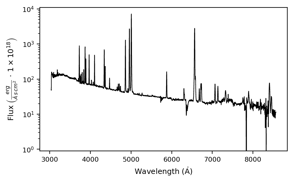
As we can see from the plot above, this object has a week continuum compared to the emission lines. To mask these features we are going to do an iterative process with the \(\tt{lime.Spectrum.fit.continuum}\) function:

gp_spec.fit.continuum(degree_list=[3, 6, 6], emis_threshold=[3, 2, 1.5], plot_steps=True, log_scale=True)

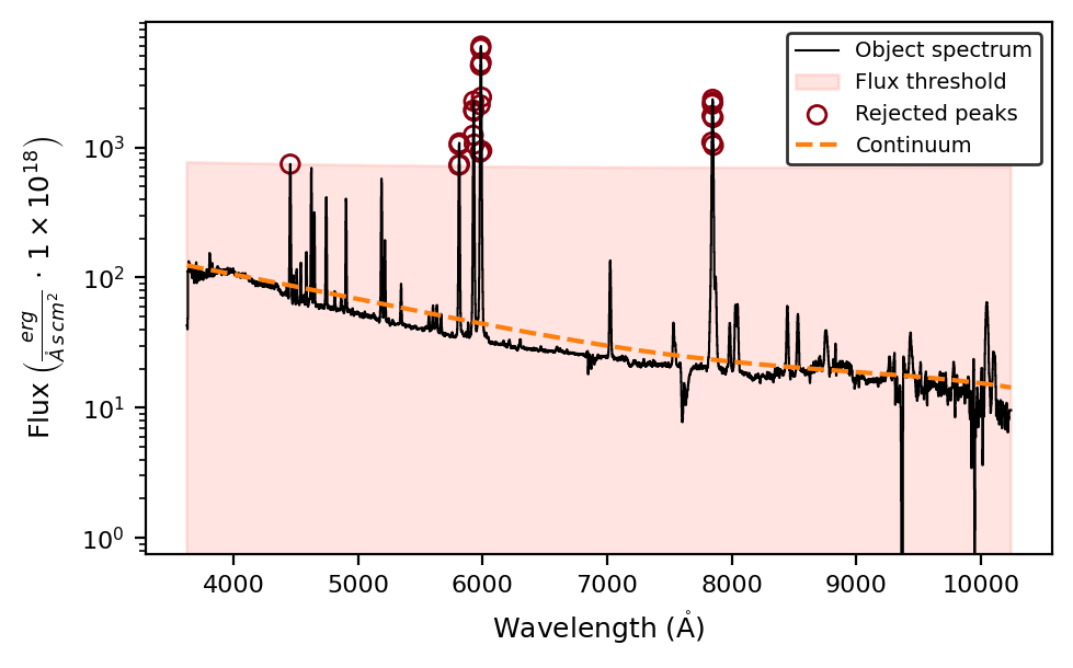
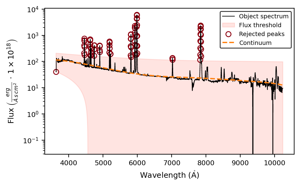
By setting plot_steps=True we can visualize the steps of the iteration. The other arguments provide additional tools to adjust the continuum fitting:

• The degree_list sets the number of iterations and the degree of the polynomial.

• The emis_threshold sets the intensity threshold for rejected pixels (marked in purple on the plots). You can also set an abs_threshold to define a lower intensity threshold. Otherwise, the same threshold will apply for pixels above and below the continuum fitting.

• The smooth_scale argument is the length in pixels for the convolve function. Smoothing the spectrum can provide a more robust estimation of the continuum.

The lime.Spectrum.cont variable stores the fitted continuum array, while the lime.Spectrum.cont_std provides the standard deviation between the observed spectrum and the fitted one.

print(gp_spec.cont)
print(gp_spec.cont_std)

[119.24158210981295 119.14751482372276 119.0532858338729 ...
 7.463363476396353 7.401425013028529 7.339188641922192]
4.099014712009923

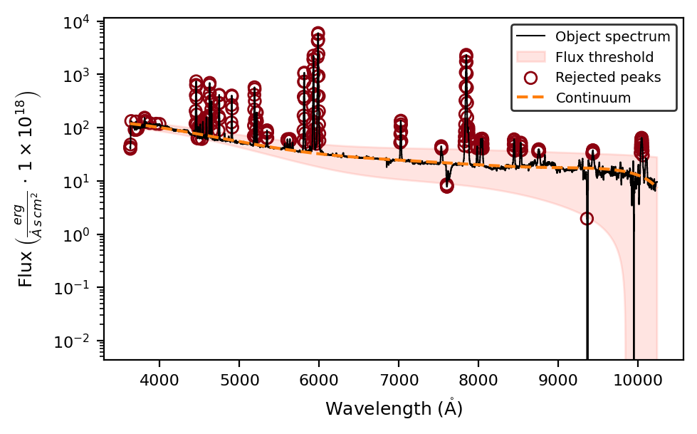
These arrays can be plotted using the \(\tt{lime.Spectrum.plot.spectrum}\) function:

gp_spec.plot.spectrum(show_cont=True, log_scale=True)

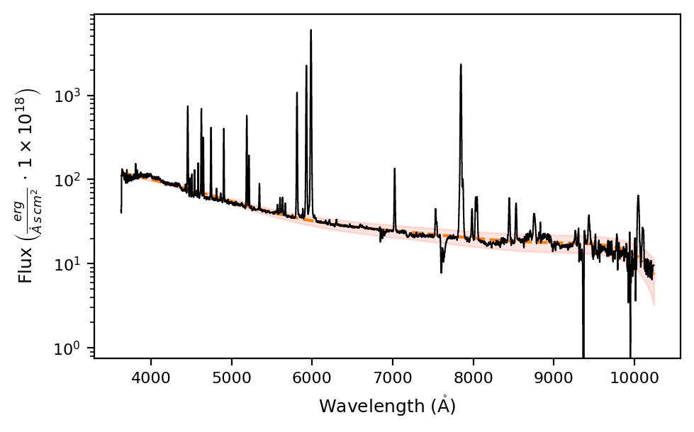
where the dashed line corresponds to lime.Spectrum.cont and the shaded area represents lime.Spectrum.cont_std.

Takeaways

• \(\mathrm{LiMe}\) provides an iterative function \(\tt{lime.Spectrum.fit.continuum}\) to fit the continuum.

• The user can provide a list with the degrees of the polynomials and the intensity thresholds for the emission and/or absorption features to be excluded at each iteration.

• The fitted continuum is stored in the \(\tt{lime.Spectrum.cont}\) attribute and is used in tasks such as line detection.

• The function arguments can be adjusted to meet the user’s needs. You can read the function documentation in the API.