Line detection

\(\mathrm{LiMe}\) includes an intensity threshold algorithm to confirm the presence of lines prior to their measurement. In this guide, we will show how the user can access these functions.

Let’s start by loading an observation:

import numpy as np
from astropy.io import fits
from pathlib import Path
import lime

# State the input files
obsFitsFile = '../0_resources/spectra/gp121903_osiris.fits'
cfgFile = '../0_resources/long_slit.toml'

# Spectrum parameters
z_obj = 0.19531
norm_flux = 1e-18

# Create the observation object
gp_spec = lime.Spectrum.from_file(obsFitsFile, instrument='osiris', redshift=z_obj, norm_flux=norm_flux)
gp_spec.plot.spectrum(log_scale=True)

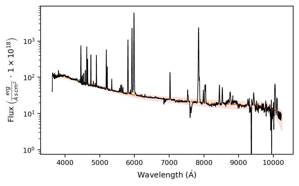
The first step is to obtain an estimate of the continuum, as demonstrated in the previous guide:

# Fit the object continuum:
gp_spec.fit.continuum(degree_list=[3, 6, 6], emis_threshold=[3, 2, 1.5])

# Plot the observation with the fitted continuum and its mean standard deviation
gp_spec.plot.spectrum(show_cont=True, log_scale=True)

Now, we retrieve a table of candidate lines for the observation wavelength range:

candidate_lines = gp_spec.retrieve.lines_frame()
candidate_lines[0:10]
print(f'{candidate_lines.index.size} candidate lines')

66 candidate lines

As you can see, this is a very large list.

It is recommended to index this table to include only the lines relevant to your astronomical study.

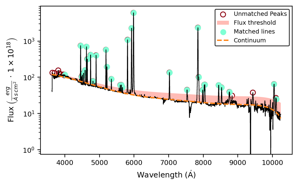
For the current guide, we will use it in the \(\tt{lime.Spectrum.infer.peaks\_troughs}\) function to match the theoretical wavelengths to the observed peaks:

matched_lines = gp_spec.infer.peaks_troughs(candidate_lines, emission_type=True, sigma_threshold=3, plot_steps=True, log_scale=True)
print(matched_lines[0:10])
print(f'{matched_lines.index.size} lines detected')

            wavelength     wave_vac           w1           w2           w3  \
Ne5_3345A  3345.400000  3346.400000  3334.246902  3338.698612  3339.336871   
H1_3722A   3721.938000  3722.997000  3665.750000  3694.260000  3715.523661   
O2_3726A   3725.974000  3727.092000  3665.750000  3694.260000  3719.555437   
O2_3729A   3728.756000  3729.875000  3665.750000  3694.260000  3722.335373   
H1_3750A   3750.092000  3751.217000  3664.503848  3675.720417  3743.650991   
H1_3771A   3770.571000  3771.701000  3758.000441  3763.017925  3764.111082   
H1_3798A   3797.838000  3798.976000  3780.949179  3792.078244  3791.352932   
H1_3835A   3835.324000  3836.472000  3823.148476  3829.538777  3828.803029   
Ne3_3869A  3869.000000  3870.160000  3848.429950  3858.099497  3862.448279   
He1_3889A  3888.584917  3889.747508  3842.087829  3861.282614  3882.014483   

                    w4           w5           w6                latex_label  \
Ne5_3345A  3351.463129  3352.089476  3356.565009    $[NeV]3345\mathring{A}$   
H1_3722A   3728.352339  3754.880000  3767.500000       $HI3750\mathring{A}$   
O2_3726A   3732.392563  3754.880000  3767.500000    $[OII]3726\mathring{A}$   
O2_3729A   3735.176627  3754.880000  3767.500000    $[OII]3729\mathring{A}$   
H1_3750A   3756.533009  3775.220000  3792.040000       $HI3750\mathring{A}$   
H1_3771A   3777.030918  3778.110650  3783.154984       $HI3771\mathring{A}$   
H1_3798A   3804.323068  3807.127865  3816.774280       $HI3798\mathring{A}$   
H1_3835A   3841.844971  3844.260000  3852.830000       $HI3835\mathring{A}$   
Ne3_3869A  3875.551721  3895.538694  3910.048413  $[NeIII]3869\mathring{A}$   
He1_3889A  3895.155351  3905.000000  3950.000000      $HeI3889\mathring{A}$   

          units_wave particle trans  rel_int observation  signal_peak  
Ne5_3345A   Angstrom      Ne5   col        0    detected        179.0  
H1_3722A    Angstrom       H1   rec        0    detected        401.0  
O2_3726A    Angstrom       O2   col        1    detected        401.0  
O2_3729A    Angstrom       O2   col        1    detected        401.0  
H1_3750A    Angstrom       H1   rec        1    detected        414.0  
H1_3771A    Angstrom       H1   rec        1    detected        426.0  
H1_3798A    Angstrom       H1   rec        1    detected        442.0  
H1_3835A    Angstrom       H1   rec        1    detected        463.0  
Ne3_3869A   Angstrom      Ne3   col        1    detected        483.0  
He1_3889A   Angstrom      He1   rec        1    detected        494.0  
41 lines detected

By setting plot_steps=True, we can visualize the steps of the iteration. The remaining arguments adjust the peak detection argument:

• The emission_shape=True sets the detection to peaks.

• The shaded area represents the sigma_threshold times spectrum.cont_std, above which peaks are detected.

• The filled circles represent the matched peaks, while the empty pale circles represent unmatched peaks. The width_tol argument sets the minimum number of pixels between peaks/troughs, with a default value of 5.

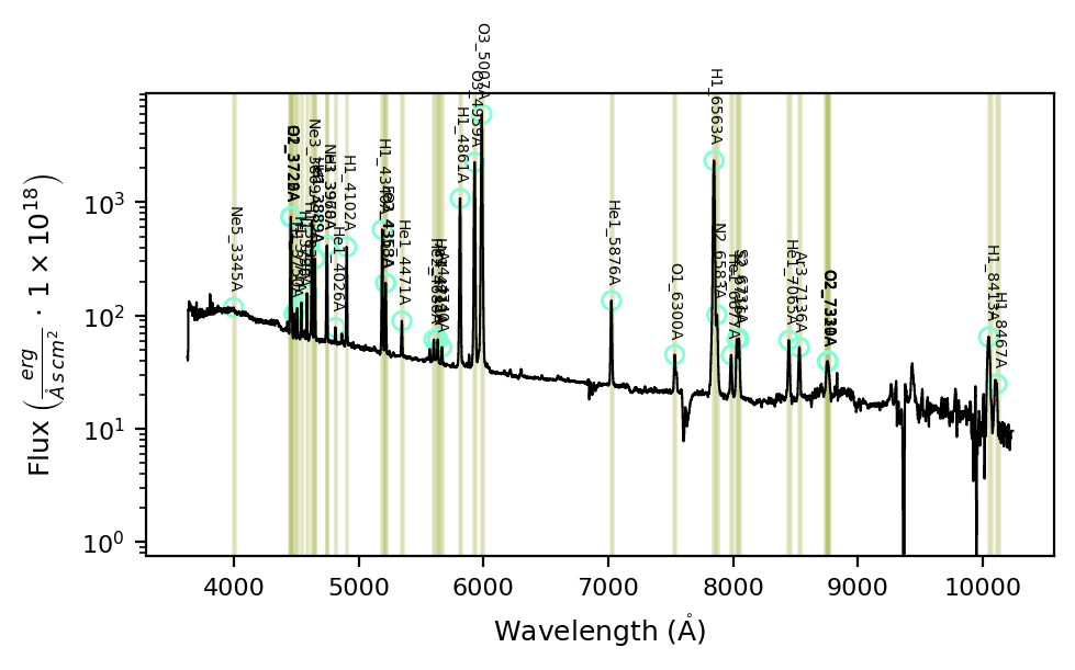
To inspect the bands, you can use the bands argument in the \(\tt{lime.Spectrum.plot.spectrum}\) function:

gp_spec.plot.spectrum(bands=matched_lines, log_scale=True)

Takeaways

• After fitting the continuum for your observation, you can run the \(\tt{lime.Spectrum.infer.peaks\_troughs}\) function to detect peaks/troughs above/below a specified multiple of the continuum flux standard deviation.

• This function compares the detected peaks/troughs against the transition wavelengths in the input bands.

• The user should ensure that the input bands are appropriate for single or blended lines.

• The function arguments can be adjusted to meet the user’s needs. You can read the function documentation in the API.