Reviewing IFS results

In this tutorial, we are going to explore some tools to check the measurements from the SHOC579 MANGA measurements.

Let’s start by loading the input and output data:

import numpy as np
import lime
from astropy.io import fits
from astropy.wcs import WCS
from matplotlib import pyplot as plt

# State the data location
cfg_file = '../0_resources/ifu_manga.toml'
cube_address = '../0_resources/spectra/manga-8626-12704-LOGCUBE.fits.gz'
bands_file_0 = '../0_resources/bands/SHOC579_MASK0_bands.txt'
spatial_mask_file = '../0_resources/results/SHOC579_mask_SN_line.fits'
output_lines_log_file = '../0_resources/SHOC579_log.fits'

# Load the configuration file:
obs_cfg = lime.load_cfg(cfg_file)

# Load the Cube
z_obj = obs_cfg['SHOC579']['redshift']
shoc579 = lime.Cube.from_file(cube_address, instrument='manga', redshift=z_obj)

WARNING: FITSFixedWarning: PLATEID = 8626 / Current plate 
a string value was expected. [astropy.wcs.wcs]
WARNING: FITSFixedWarning: 'datfix' made the change 'Set MJD-OBS to 57277.000000 from DATE-OBS'. [astropy.wcs.wcs]

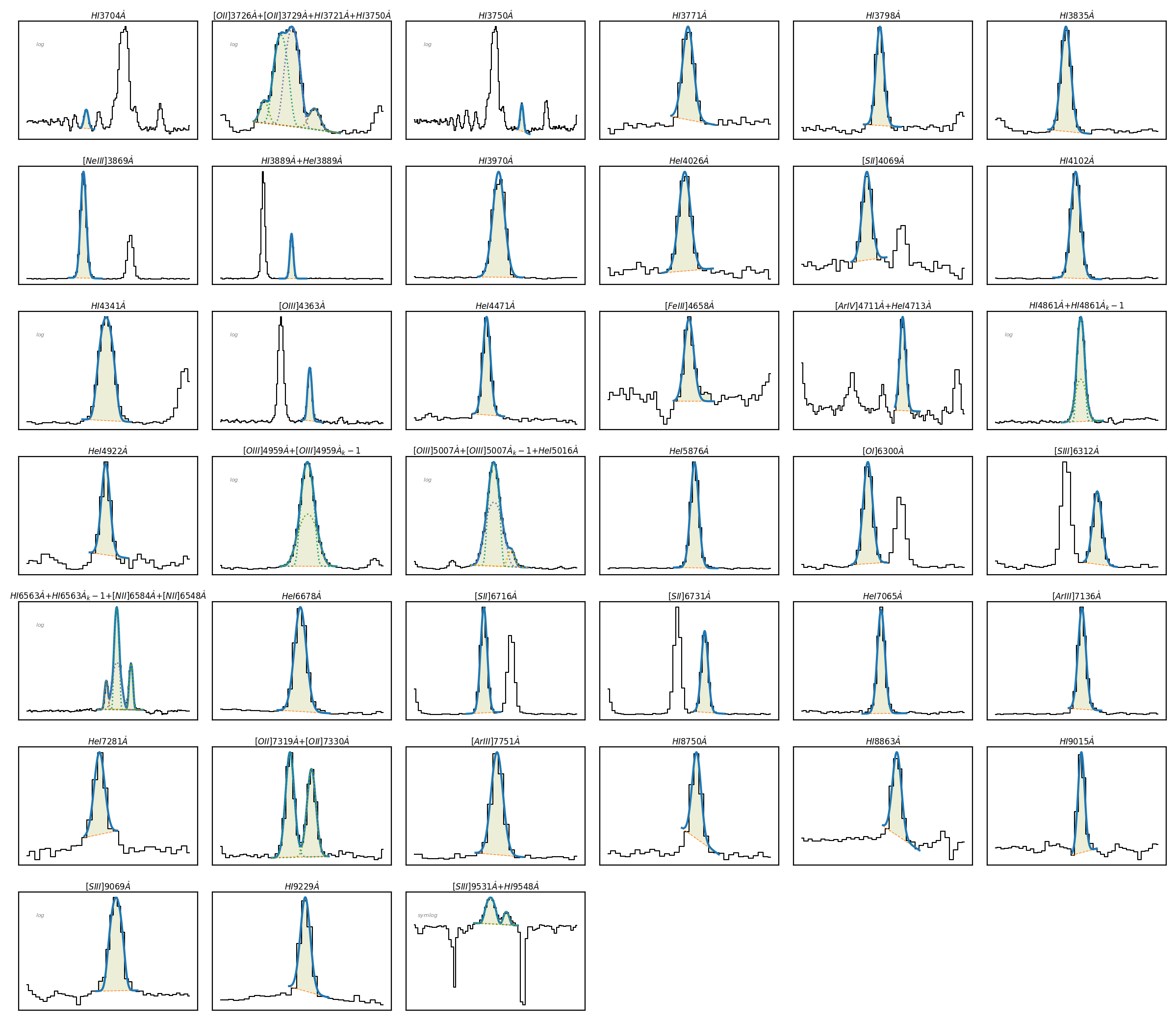
If we include the lines_file argument in the \(\tt{lime.Cube.check.cube}\) function you can review the spaxel spectrum with the fitted profiles:

shoc579.check.cube('H1_6563A', fname=output_lines_log_file, masks_file=spatial_mask_file)

/home/vital/anaconda3/envs/lime2/lib/python3.12/site-packages/numpy/lib/_function_base_impl.py:4859: UserWarning: Warning: 'partition' will ignore the 'mask' of the MaskedArray.
  arr.partition(

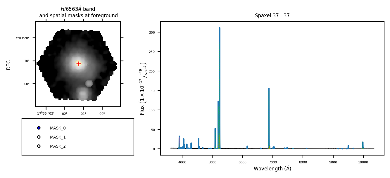
Or you can load the measurements from individual spaxels:

# Check the individual spaxel fitting configuration
spaxel = shoc579.get_spectrum(38, 35)
spaxel.load_frame(output_lines_log_file, page='38-35_LINELOG')
spaxel.plot.grid()

Spatial parameter maps

The \(\tt{lime.save\_parameter\_maps}\) can extract the parameter maps as multi-page .fits file:

# Export the line measurements as spatial maps:
param_list = ['intg_flux', 'intg_flux_err', 'profile_flux', 'profile_flux_err', 'v_r', 'v_r_err']
lines_list = ['H1_4861A', 'H1_6563A', 'O3_4363A', 'O3_4959A', 'O3_5007A', 'S3_6312A', 'S3_9069A', 'S3_9531A']
lime.save_parameter_maps(output_lines_log_file, '../0_resources/', param_list, lines_list,
                         mask_file=spatial_mask_file, output_file_prefix='SHOC579_', wcs=shoc579.wcs)

[==========] 100% of spaxels from file "../0_resources/SHOC579_log.fits" read (227 total)

Please remember: The inputs and outputs of the lime.save_parameter_maps can only be .fits files and the mask_file argument is necessary to make sure only the spaxels with scientific data are considered

This function produces different outputs depending on its arguments:

• The param_list argument establishes which parameters from the input output_lines_log_file will be exported into a .fits file. There will be .fits file per item on the param_list. These files will be stored on the output_folder using output_files_prefix and the item name. The item name must follow the parameter notation of the logs measurements.

• The line_list arguments establishes, which line measurements are exported to the output parameter .fits files. Each file will have one extension per line.

• The user can specify a binary mask with the mask_file argument. By default default it will use all the masks extensions on the input .fits unless the user specifies certain masks with the mask_list argument.

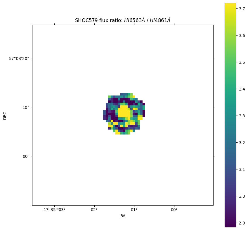
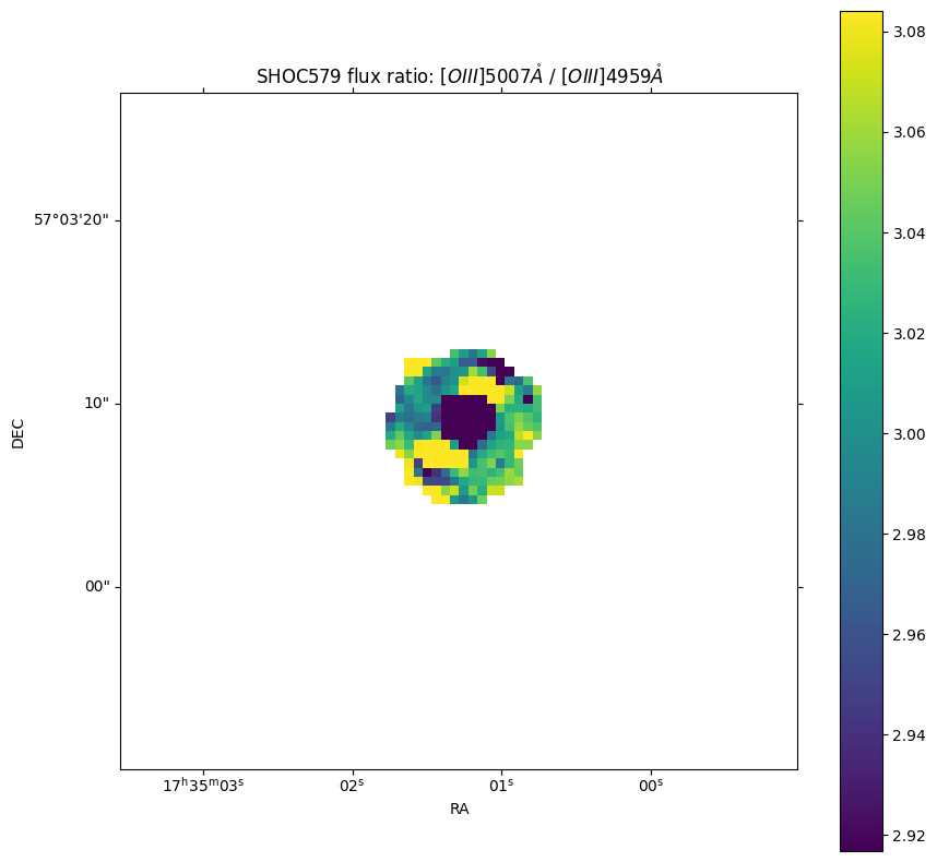
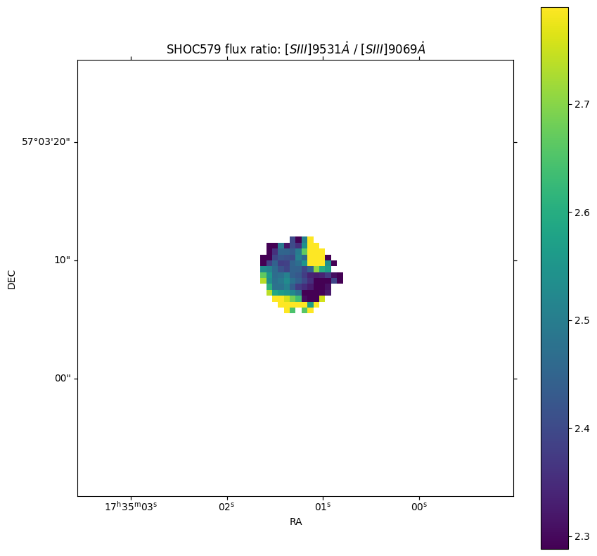
At this point we plot some flux ratio diagnostics from theses maps. Let’s define them:

# State line ratios for the plots
lines_ratio = {'H1': ['H1_6563A', 'H1_4861A'],
               'O3': ['O3_5007A', 'O3_4959A'],
               'S3': ['S3_9531A', 'S3_9069A']}

# State the parameter map file
fits_file = f'../0_resources/SHOC579_profile_flux.fits'

# Loop through the line ratios
for ion, lines in lines_ratio.items():

    # Recover the parameter measurements
    latex_array = lime.label_decomposition(lines, params_list=['latex_label'])[0]
    ratio_map = fits.getdata(fits_file, lines[0]) / fits.getdata(fits_file, lines[1])
    Halpha = fits.getdata(fits_file, lines[0])
    Hbeta = fits.getdata(fits_file, lines[1])

    # Get the astronomical coordinates from one of the headers of the lines log
    hdr = fits.getheader(fits_file, lines[0])
    wcs_maps = WCS(hdr)

    # Create the plot
    fig = plt.figure(figsize=(10, 10))
    ax = fig.add_subplot(projection=wcs_maps, slices=('x', 'y'))
    im = ax.imshow(ratio_map, vmin=np.nanpercentile(ratio_map, 16), vmax=np.nanpercentile(ratio_map, 84))
    cbar = fig.colorbar(im, ax=ax)
    ax.update({'title': f'SHOC579 flux ratio: {latex_array[0]} / {latex_array[1]}', 'xlabel': r'RA', 'ylabel': r'DEC'})
    plt.show()

Take aways

• The \(\tt{lime.Cube.check.cube}\) function can be used to checked the fitted line profiles by using the lines_file argument. Similarly you can extract individual spectra using \(\tt{lime.Cube.get\_spectrum}\) the function and loading the spaxel measurements using \(\tt{lime.Spectrum.load\_frame}\).

• The \(\tt{lime.save\_parameter\_maps}\) function can generate spatial parameters from the requested params as a multi-page fits file.

• You can read the function documentation in the API.