Preparing the lines table#
It is recommended that you prepare a generic line bands table containing the lines you expect to find in your astronomical objects and scientific projects.
Afterward, you can tailor this template to the specific features and artifacts present in each spectrum as needed.
Generic lines template#
You can adjust \(\mathrm{LiMe}\) lines database using the \(\texttt{lime.lines\_frame}\) function.
from pathlib import Path
import lime


# State the data files
cfgFile = '../0_resources/long_slit.toml'
obsFitsFile = '../0_resources/spectra/gp121903_osiris.fits'
osiris_gp_df_path = Path('../0_resources/bands/osiris_green_peas_linesDF.txt')
gp121903_df_path = '../0_resources/bands/gp121903_bands.txt'

# Load configuration
obs_cfg = lime.load_cfg(cfgFile)

# Prepare lines template for emission lines galaxy
osiris_gp_df = lime.lines_frame(wave_intvl=[3000, 10000],
                                rejected_lines=['H1_3722A', 'H1_3734A', 'Fe3_4008A', 'S2_4076A',
                                               'Fe2_4358A', 'Fe3_4881A', 'Ar3_5192A'])
lime.save_frame(osiris_gp_df_path, osiris_gp_df)

print(osiris_gp_df)
           wavelength  wave_vac           w1           w2           w3  \
Ne5_3345A    3345.400  3346.400  3334.246902  3338.698612  3340.936379
Ne5_3426A    3425.500  3426.500  3390.000000  3410.000000  3420.929505
H1_3704A     3703.794  3704.906  3671.309441  3681.364925  3698.852189
O2_3726A     3725.974  3727.092  3665.750000  3694.260000  3721.002595
O2_3729A     3728.756  3729.875  3665.750000  3694.260000  3723.780884
...               ...       ...          ...          ...          ...
H1_9015A     9014.774  9017.385  8975.870000  9001.890000  9002.745980
S3_9068A     9068.500  9071.100  9028.280000  9056.360000  9056.400296
H1_9229A     9228.875  9231.547  9198.107216  9210.388042  9216.561315
S3_9530A     9530.400  9533.200  9471.122554  9489.978978  9517.684003
H1_9546A     9545.830  9548.590  9471.122554  9489.978978  9533.093415

                    w4           w5           w6               latex_label  \
Ne5_3345A  3349.863621  3352.089476  3356.565009   $[NeV]3345\mathring{A}$
Ne5_3426A  3430.070495  3445.000000  3465.000000   $[NeV]3426\mathring{A}$
H1_3704A   3708.735811  3758.000000  3764.000000      $HI3704\mathring{A}$
O2_3726A   3730.945405  3754.880000  3767.500000   $[OII]3726\mathring{A}$
O2_3729A   3733.731116  3754.880000  3767.500000   $[OII]3729\mathring{A}$
...                ...          ...          ...                       ...
H1_9015A   9026.802020  9029.944250  9048.681886      $HI9015\mathring{A}$
S3_9068A   9080.599704  9083.325784  9100.603298  $[SIII]9068\mathring{A}$
H1_9229A   9241.188685  9247.329098  9259.675643      $HI9229\mathring{A}$
S3_9530A   9543.115997  9569.193420  9600.501253  $[SIII]9530\mathring{A}$
H1_9546A   9558.566585  9569.193420  9600.501253      $HI9546\mathring{A}$

          units_wave particle trans  rel_int
Ne5_3345A   Angstrom      Ne5   col        0
Ne5_3426A   Angstrom      Ne5   col        0
H1_3704A    Angstrom       H1   rec        1
O2_3726A    Angstrom       O2   col        1
O2_3729A    Angstrom       O2   col        1
...              ...      ...   ...      ...
H1_9015A    Angstrom       H1   rec        1
S3_9068A    Angstrom       S3   col        1
H1_9229A    Angstrom       H1   rec        1
S3_9530A    Angstrom       S3   col        1
H1_9546A    Angstrom       H1   rec        1

[68 rows x 13 columns]
Object lines template#
If you create a \(\texttt{lime.Spectrum}\):
# Load observation data
z_obj = obs_cfg['osiris']['gp121903']['z']
norm_flux = obs_cfg['osiris']['norm_flux']
gp_spec = lime.Spectrum.from_file(obsFitsFile, instrument='osiris', redshift=z_obj, norm_flux=norm_flux)
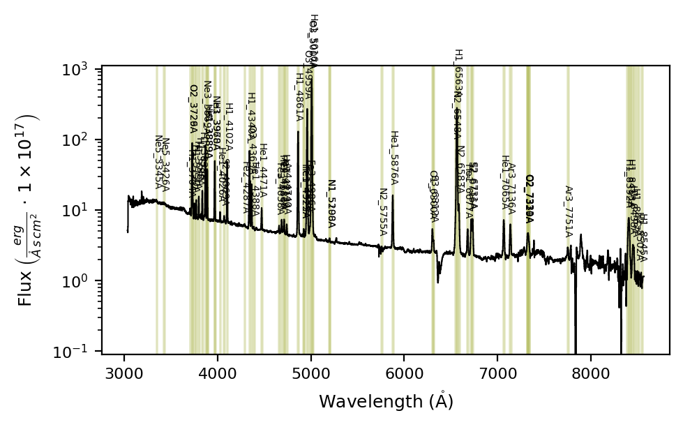
You can use \(\texttt{lime.Spectrum.retrieve.lines\_frame}\) to further adjust the default or input lines frame to match your observation:
# Generate the object lines table from the previous template
obj_linesDF = gp_spec.retrieve.lines_frame(ref_bands=osiris_gp_df_path)
gp_spec.plot.spectrum(bands=obj_linesDF, log_scale=True, rest_frame=True)
The \(\texttt{lime.Spectrum.retrieve.lines\_frame}\) function shares most arguments with \(\texttt{lime.lines\_frame}\) (except for wave_intvl and redshift, which are taken from the spectrum), and also provides additional arguments to group the lines.
Explicit grouping:#
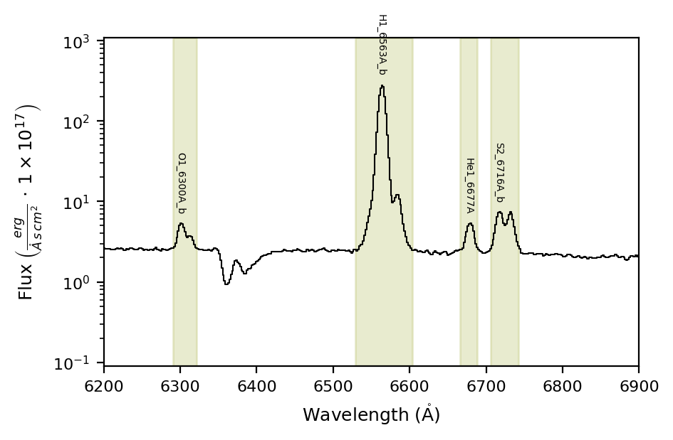
If you provide a configuration file or dictionary in fit_cfg, the function will check it for merged and blended lines and include them in the output lines frame:
# Generate the object lines table from the previous template
obj_linesDF = gp_spec.retrieve.lines_frame(band_vsigma=100, n_sigma=4, instrumental_correction=True,
                                           map_band_vsigma={'H1_4861A': 200, 'H1_6563A': 200,
                                                            'N2_6548A': 200, 'N2_6583A': 200,
                                                            'O3_4959A': 250, 'O3_5007A': 250},
                                           fit_cfg={'O2_3726A_m': 'O2_3726A+O2_3729A',
                                                          'H1_3889A_m': "H1_3889A+He1_3889A",
                                                          'Ne3_3968A_m': "Ne3_3968A+H1_3970A",
                                                          'Ar4_4711A_m': "Ar4_4711A+He1_4713A",
                                                          'Fe3_4925A_m': 'He1_4922A+Fe3_4925A',
                                                          'N1_5198A_m': "N1_5198A+N1_5200A",
                                                          'O1_6300A_b': "O1_6300A+S3_6312A",
                                                          'H1_6563A_b': "H1_6563A+N2_6583A+N2_6548A",
                                                          'S2_6716A_b': "S2_6716A+S2_6731A"},
                                           ref_bands=osiris_gp_df_path)

gp_spec.plot.spectrum(bands=obj_linesDF, log_scale=True, rest_frame=True, in_fig=None)
gp_spec.plot.ax.set_xlim(6200, 6900)
gp_spec.plot.show()
You can constrain the grouped lines from fit_cfg to a sublist using the grouped_lines argument:
# Generate the object lines table from the previous template
obj_linesDF = gp_spec.retrieve.lines_frame(band_vsigma=100, n_sigma=4, instrumental_correction=True,
                                           map_band_vsigma={'H1_4861A': 200, 'H1_6563A': 200,
                                                            'N2_6548A': 200, 'N2_6583A': 200,
                                                            'O3_4959A': 250, 'O3_5007A': 250},
                                           fit_cfg=obs_cfg,
                                           grouped_lines=['O1_6300A_b'],
                                           ref_bands=osiris_gp_df_path)

gp_spec.plot.spectrum(bands=obj_linesDF, log_scale=True, rest_frame=True, in_fig=None)
gp_spec.plot.ax.set_xlim(6200, 6900)
gp_spec.plot.show()
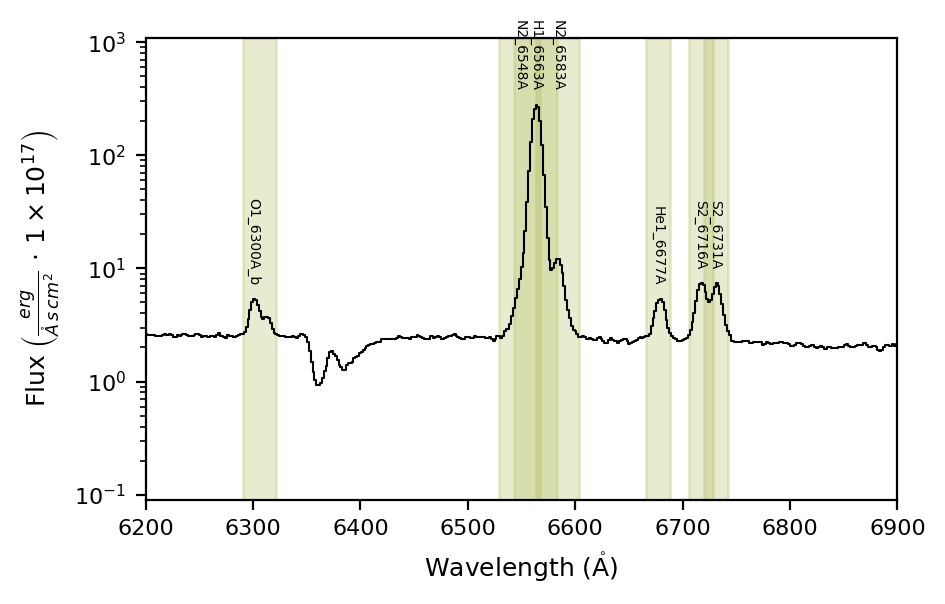
In this case only O1_6300A_b is grouped:
obj_linesDF.iloc[27:45]
| wavelength | wave_vac | w1 | w2 | w3 | w4 | w5 | w6 | latex_label | units_wave | particle | trans | rel_int | |
|---|---|---|---|---|---|---|---|---|---|---|---|---|---|
| H1_4861A | 4861.2500 | 4862.6830 | 4809.800000 | 4836.100000 | 4845.338856 | 4877.161144 | 4883.130000 | 4908.400000 | $HI4861\mathring{A}$ | Angstrom | H1 | rec | 1 |
| He1_4922A | 4922.3330 | 4923.7830 | 4905.922627 | 4912.472756 | 4912.827226 | 4931.838774 | 4932.175718 | 4938.760898 | $HeI4922\mathring{A}$ | Angstrom | He1 | rec | 1 |
| Fe3_4925A | 4924.5800 | 4926.0310 | 4908.162136 | 4914.715255 | 4915.070920 | 4934.089080 | 4934.427211 | 4941.015398 | $[FeIII]4925\mathring{A}$ | Angstrom | Fe3 | col | 1 |
| O3_4959A | 4958.8350 | 4960.2950 | 4929.281844 | 4946.732665 | 4939.355882 | 4978.314118 | 4972.820372 | 4984.416360 | $[OIII]4959\mathring{A}$ | Angstrom | O3 | col | 1 |
| Fe3_4986A | 4985.8000 | 4987.2700 | 4969.178037 | 4975.812621 | 4976.208839 | 4995.391161 | 4995.769627 | 5002.439715 | $[FeIII]4986\mathring{A}$ | Angstrom | Fe3 | col | 0 |
| O3_5007A | 5006.7700 | 5008.2400 | 4971.796688 | 4984.514249 | 4987.131280 | 5026.408720 | 5027.743260 | 5043.797081 | $[OIII]5007\mathring{A}$ | Angstrom | O3 | col | 1 |
| He1_5016A | 5015.6000 | 5017.0800 | 4998.878688 | 5005.552927 | 5005.969864 | 5025.230136 | 5025.629215 | 5032.339170 | $HeI5016\mathring{A}$ | Angstrom | He1 | rec | 1 |
| N1_5198A | 5197.8220 | 5199.3490 | 5180.493185 | 5187.409906 | 5187.948388 | 5207.695612 | 5208.215587 | 5215.169321 | $[NI]5198\mathring{A}$ | Angstrom | N1 | col | 1 |
| N1_5200A | 5200.1776 | 5201.7055 | 5182.840932 | 5189.760787 | 5190.300492 | 5210.054708 | 5210.575898 | 5217.532783 | $[NI]5200\mathring{A}$ | Angstrom | N1 | col | 1 |
| N2_5755A | 5754.5600 | 5756.2400 | 5700.000000 | 5720.000000 | 5743.943695 | 5765.176305 | 5800.000000 | 5820.000000 | $[NII]5755\mathring{A}$ | Angstrom | N2 | col | 1 |
| He1_5876A | 5875.5352 | 5877.2535 | 5845.715833 | 5865.712378 | 5864.757537 | 5886.312863 | 5888.378245 | 5901.854752 | $HeI5876\mathring{A}$ | Angstrom | He1 | rec | 1 |
| O1_6300A_b | 6300.2080 | 6302.0460 | 6270.921363 | 6282.896208 | 6288.863300 | 6323.360285 | 6326.667186 | 6338.205448 | $[OI]6300\mathring{A}$+$[SIII]6312\mathring{A}$ | Angstrom | O1 | col | 1 |
| N2_6548A | 6547.9400 | 6549.8500 | 6480.030000 | 6520.660000 | 6527.527976 | 6568.352024 | 6627.700000 | 6661.820000 | $[NII]6548\mathring{A}$ | Angstrom | N2 | col | 1 |
| H1_6563A | 6562.7000 | 6564.6100 | 6480.030000 | 6520.660000 | 6542.248952 | 6583.151048 | 6627.700000 | 6661.820000 | $HI6563\mathring{A}$ | Angstrom | H1 | rec | 1 |
| N2_6583A | 6583.3600 | 6585.2800 | 6480.030000 | 6520.660000 | 6562.853864 | 6603.866136 | 6627.700000 | 6661.820000 | $[NII]6583\mathring{A}$ | Angstrom | N2 | col | 1 |
| He1_6677A | 6676.8753 | 6678.8205 | 6654.615528 | 6663.500418 | 6665.028235 | 6688.722365 | 6690.226409 | 6699.158845 | $HeI6677\mathring{A}$ | Angstrom | He1 | rec | 1 |
| S2_6716A | 6716.3300 | 6718.2900 | 6686.785257 | 6706.310255 | 6704.430437 | 6728.229563 | 6744.438091 | 6759.956250 | $[SII]6716\mathring{A}$ | Angstrom | S2 | col | 1 |
| S2_6731A | 6730.7100 | 6732.6700 | 6686.785257 | 6706.310255 | 6718.791014 | 6742.628986 | 6744.438091 | 6759.956250 | $[SII]6731\mathring{A}$ | Angstrom | S2 | col | 1 |
Automatic grouping:#
In the scenario where you have many observations with variable resolving power, certain transitions can be merged or blended.
\(\mathrm{LiMe}\) can review the spectral bands and the pixel width of the spectrum to get the best group for each observation. In this case you need to set the argument automatic_grouping=True.
For example, our configuration file has a blended and merged groups for the same lines (such as S2_6716A_b/S2_6716A_m or H1_6563A_m/H1_6563A_b)
obs_cfg['default_line_fitting']
{'transitions': {'O2_3726A_m': {'wavelength': 3728.484},
  'O2_7325A_m': {'wavelength': 7325.0},
  'O2_7325A_b': {'wavelength': 7325.0}},
 'O2_3726A_m': 'O2_3726A+O2_3729A',
 'O2_3726A_b': 'O2_3726A+O2_3729A',
 'H1_3889A_m': 'H1_3889A+He1_3889A',
 'Ne3_3968A_m': 'Ne3_3968A+H1_3970A',
 'Ar4_4711A_m': 'Ar4_4711A+He1_4713A',
 'Fe3_4925A_m': 'He1_4922A+Fe3_4925A',
 'O3_5007A_m': 'O3_4959A+O3_5007A',
 'O3_5007A_b': 'O3_4959A+O3_5007A',
 'N1_5198A_m': 'N1_5198A+N1_5200A',
 'O1_6300A_b': 'O1_6300A+S3_6312A',
 'H1_6563A_m': 'H1_6563A+N2_6583A+N2_6548A',
 'H1_6563A_b': 'H1_6563A+N2_6583A+N2_6548A',
 'S2_6716A_b': 'S2_6716A+S2_6731A',
 'S2_6716A_m': 'S2_6716A+S2_6731A',
 'O2_7325A_b': 'O2_7319A_m+O2_7330A_m',
 'O2_7325A_m': 'O2_7319A_m+O2_7330A_m',
 'O2_7319A_m': 'O2_7319A+O2_7320A',
 'O2_7330A_m': 'O2_7330A+O2_7331A',
 'continuum': {'degree_list': [3, 6, 6], 'emis_threshold': [3, 2, 1.5]},
 'peaks_troughs': {'sigma_threshold': 3}}
So if we run:
# Generate the object lines table from the previous template
obj_linesDF = gp_spec.retrieve.lines_frame(band_vsigma=100, n_sigma=4, instrumental_correction=True,
                                           map_band_vsigma={'H1_4861A': 200, 'H1_6563A': 200,
                                                            'N2_6548A': 200, 'N2_6583A': 200,
                                                            'O3_4959A': 250, 'O3_5007A': 250},
                                           fit_cfg=obs_cfg,
                                           automatic_grouping=True,
                                           ref_bands=osiris_gp_df_path)

gp_spec.plot.spectrum(bands=obj_linesDF, log_scale=True, rest_frame=True, in_fig=None)
gp_spec.plot.ax.set_xlim(6200, 7500)
gp_spec.plot.show()
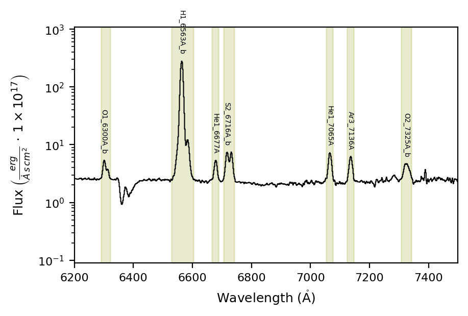
The correct line groups have been properly selected.
Please note: In addition to the Rayleigh_threshold argument, the order of the groups in the input configuration affects the grouping algorithm. For example, H1_6563A_m=‘H1_6563A+N2_6583A+N2_6548A’ is evaluated before H1_6563A_b=‘H1_6563A+N2_6583A+N2_6548A’. This can be used as a mechanism to give certain groups higher priority.
Additionally, the current automatic grouping does not take kinematic components into consideration, and these components will be excluded from the group. Please check this function’s documentation for further insight.
Advanced grouping#
The \(\texttt{lime.Spectrum.retrieve.lines\_frame}\) accepts multiple levels, as in the case of multi-object fitting, you can provide local object section from the configuration file to update (default) or overwrite the input configuration.
For example in our configuration file we have a section with additional settings:
obs_cfg['gp121903_osiris_line_fitting']
{'grouped_lines': ['O3_5007A_b', 'O3_4959A_b'],
 'rejected_lines': ['H1_3722A',
  'H1_3734A',
  'Fe3_4008A',
  'S2_4076A',
  'Fe2_4358A',
  'Fe3_4881A',
  'Fe3_4881A',
  'Fe3_4986A',
  'He1_5016A',
  'Ar3_5192A',
  'H1_8392A',
  'H1_8413A',
  'H1_8438A',
  'H1_8467A',
  'H1_8502A',
  'H1_8545A'],
 'map_band_vsigma': {'H1_4861A': 200,
  'H1_6563A': 200,
  'N2_6548A': 200,
  'N2_6583A': 200,
  'O3_4959A': 250,
  'O3_5007A': 250},
 'O3_4959A_b': 'O3_4959A+O3_4959A_k-1',
 'O3_4959A_k-1_amp': {'expr': '<100.0*O3_4959A_amp', 'min': 0.0},
 'O3_4959A_k-1_sigma': {'expr': '>2.0*O3_4959A_sigma'},
 'O3_5007A_b': 'O3_5007A+O3_5007A_k-1',
 'O3_5007A_k-1_amp': {'expr': '<100.0*O3_5007A_amp', 'min': 0.0},
 'O3_5007A_k-1_sigma': {'expr': '>2.0*O3_5007A_sigma'},
 'H1_6563A_b': 'H1_6563A+N2_6583A+N2_6548A',
 'N2_6548A_amp': {'expr': 'N2_6583A_amp/2.94'},
 'N2_6548A_kinem': 'N2_6583A',
 'S2_6716A_b': 'S2_6716A+S2_6731A',
 'S2_6731A_kinem': 'S2_6716A',
 'O2_7330A_m_kinem': 'O2_7319A_m'}
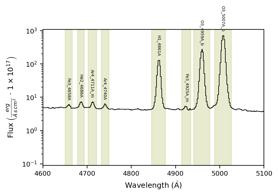
If we include the section prefix in the obj_cfg_prefix argument, we can further adjust the bands for this object:
# Generate the object lines table from the previous template
obj_linesDF = gp_spec.retrieve.lines_frame(band_vsigma=100, n_sigma=4, instrumental_correction=True,
                                           map_band_vsigma={'H1_4861A': 200, 'H1_6563A': 200,
                                                            'N2_6548A': 200, 'N2_6583A': 200,
                                                            'O3_4959A': 250, 'O3_5007A': 250},
                                           fit_cfg=obs_cfg, obj_cfg_prefix='gp121903_osiris',
                                           automatic_grouping=True,
                                           ref_bands=osiris_gp_df_path)

gp_spec.plot.spectrum(bands=obj_linesDF, log_scale=True, rest_frame=True, in_fig=None)
gp_spec.plot.ax.set_xlim(4600, 5100)
gp_spec.plot.show()
lime.save_frame(gp121903_df_path, obj_linesDF)
Several things are happening here:
The
rejected_linesare automatically read from the input configuration (that’s why we don’t have Fe3_4986A or He1_5016A now).The
grouped_linesare also read from the input configuration. However, because we are using theautomatic_grouping=Trueargument, the other lines are considered as well, although thegrouped_linestake priority.The current automatic grouping does not take kinematic components into consideration. Therefore, we set
grouped_lines = ['O3_5007A_b', 'O3_4959A_b']to force these groups in the output line bands.
Takeaways#
Start by generating a lines template for your current project instrument and scientific targets. You can get a copy of the default \(\mathrm{LiMe}\) database using the \(\texttt{lime.lines\_frame}\) function.
Use this template as the
ref_bandsin your observation with the \(\texttt{lime.Spectrum.retrieve.lines\_frame}\) function.Depending on the number of spectra you need to analyze, this function provides several arguments to tailor the output bands:
Specify the line groups you want with the
fit_cfgargument.Provide all candidate groups you may observe in
fit_cfgand then setautomatic_grouping=Truefor automatic grouping.Combine both approaches with multiple levels in
fit_cfgto set a default behavior for your sample and alocalconfiguration with theobj_cfg_prefix.Currently, automatic grouping does not consider kinematic components. Therefore, you must set them in the
grouped_linesargument (or fitting configuration file) to make them available when usingautomatic_grouping=True.
Check the API for more details on these functions.