%matplotlib widget

Line labels

The first input for measurements is the label for the line being measured. Our notation follows the style used by the PyNeb library package by V. Luridiana, C. Morisset and R. A. Shaw (2015).

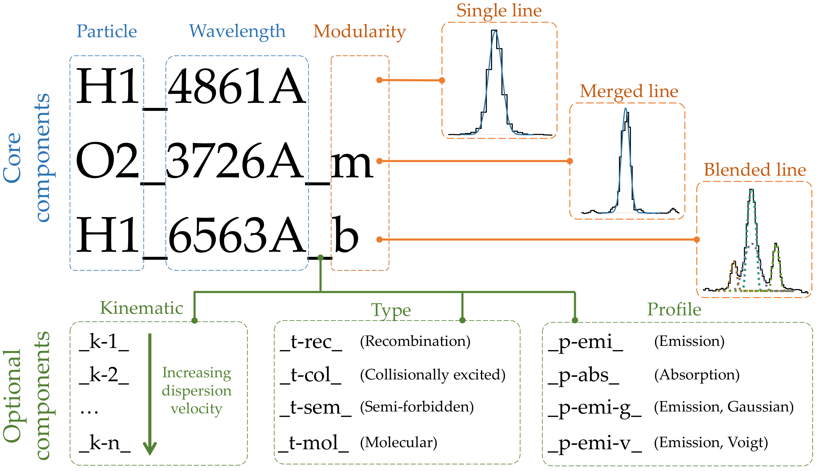
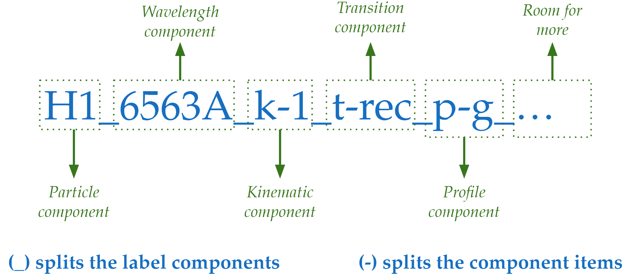
The core elements are the particle responsible for the transition, the transition wavelength (with its units) and the profile modularity.

Additional suffixes provide additional information for the transition properties and/or profile fitting conditions. The image below shows some example:

# # Import libraries for the example
# from IPython.display import Image, display
# import lime

# display(Image(filename='../images/label_components.png', width = 1200))

Core components

These are the compulsory elements of the label whose order is fixed.

1) Particle component

The first component of the line label is the particle responsible for the transition

By default expects the particle chemical symbol followed by the ionization state in Arabic numerals. If the particle is recognized, its mass will be used to compute the thermal dispersion velocity in the output measurements. The user can add additional details to the transition by via dashses.

For example: H1_18750A, H1-PashchenAlpha_1875nm, or H1-4-3_1875.0nm are all processed similarly.

2) Wavelength component

The second item is the transition wavelength. This positive real number must be followed by the transition’s wavelength or frequency units. These units must follow AstroPy notation, with the exception of the Angstroms which can be defined with an “A”, in addition to “AA” or “Angstrom””.

Please remember: assumes that this wavelength is in the restframe.

3) Modularity component

The final core component informs if the line profile fitting consists in one or multiple profiles. This item must be at the end of the line label string. The following images provide show examples of for the three type of modules for the fitting of the same transitions the doublet:

Single line

A single emission or absorption line can be modeled with a single profile:

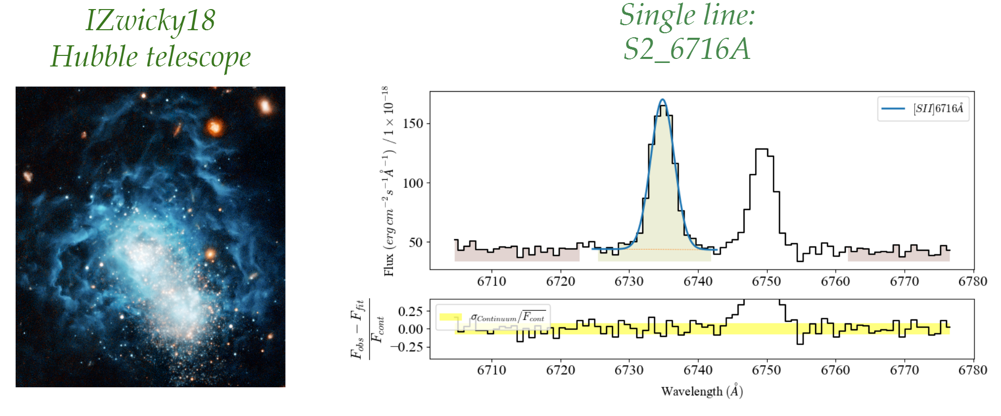
This is the default profile fitting and no suffix is required.

Blended line

A blended line consists in several transtions and/or kinematic components. If the user adds the the *”_b”* suffix and includes the components in the fitting configuration (joined by “+”). will proceed to fit one profile per component:

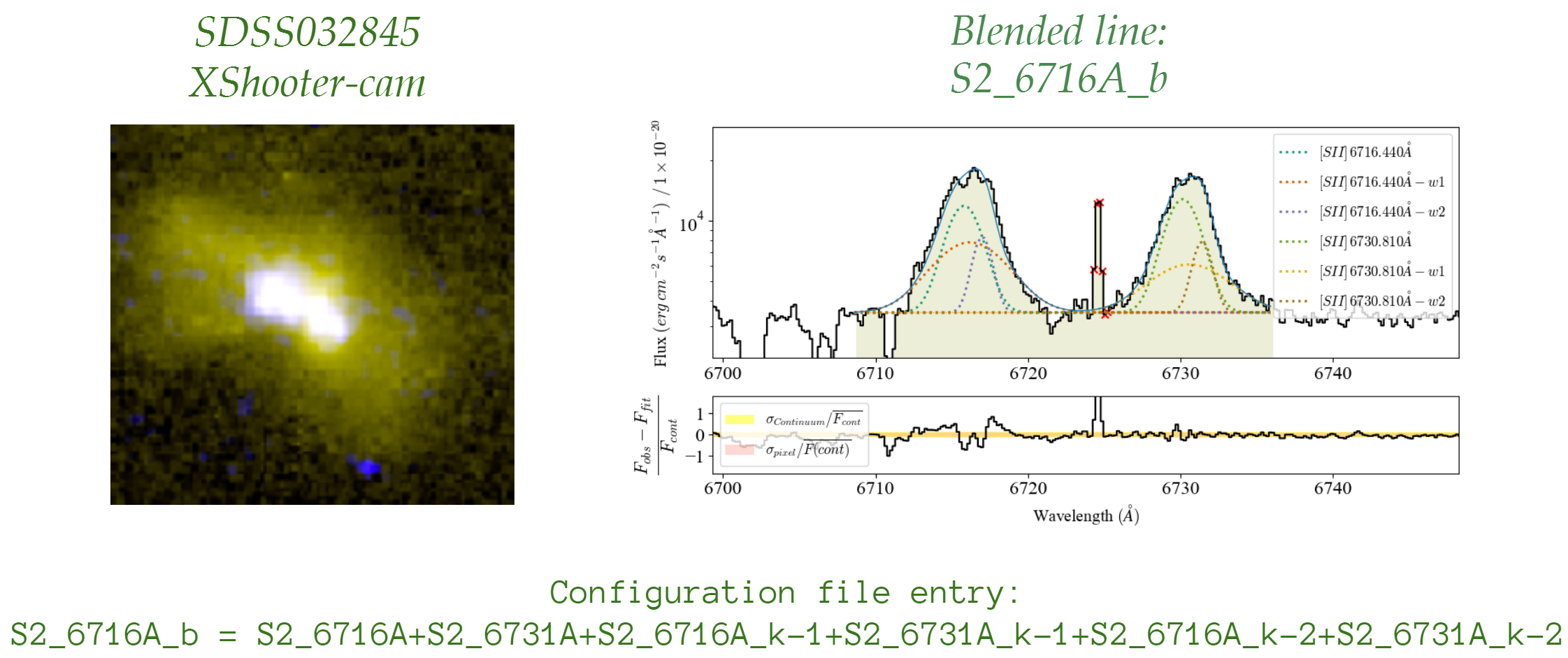
In the example, we fit both transitions, where each line has 2 additional kinematic components. These kinematic components must include the kinematic suffix (_k-1, _k-2, …).

Merged line

A merged line assumes that there are multiple transition contributing to the observed line but only one profile is fitted. If the user adds the *”_m”* suffix and includes the components in the fitting configuration (joined by “+”) these components will be included alongside the line measurements.

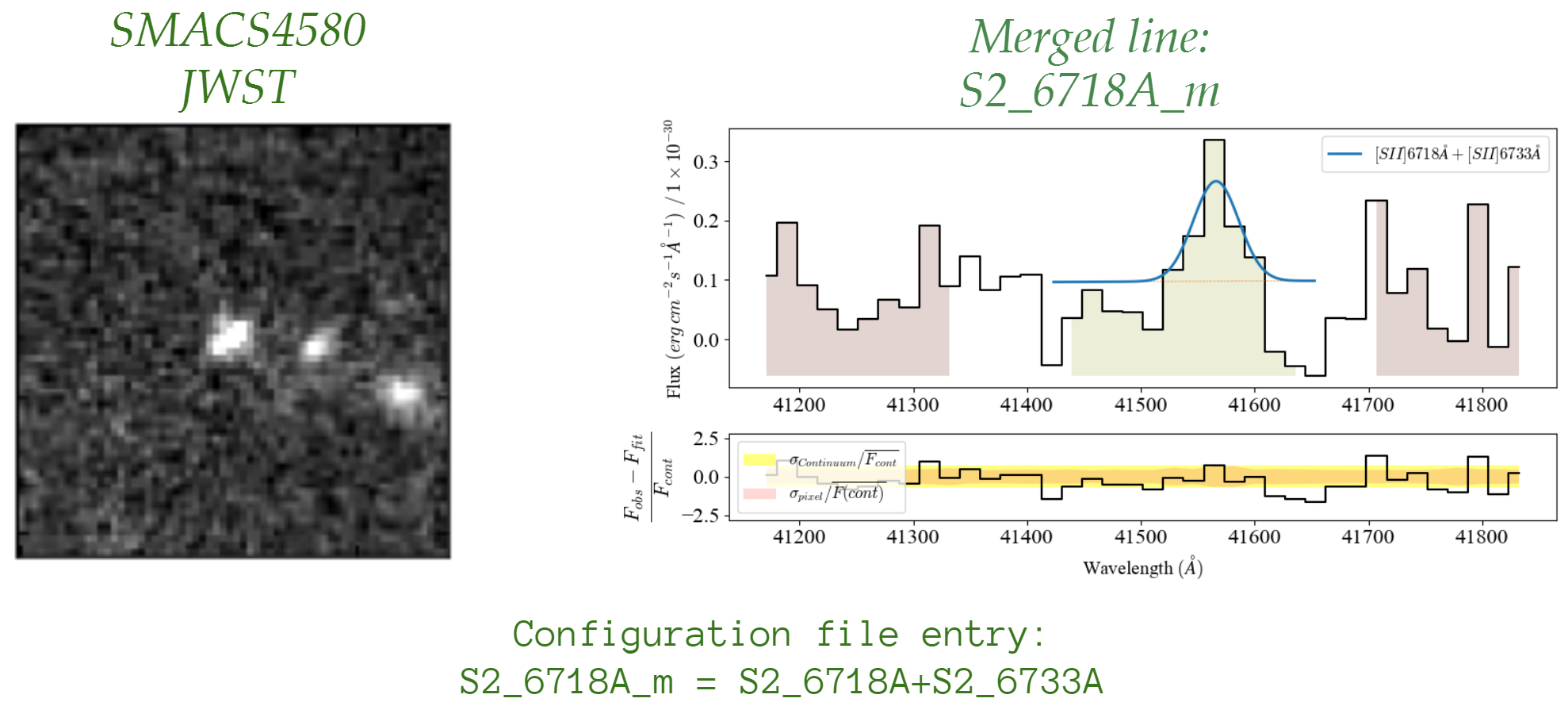
This classification is useful in those cases where the user wants to keep track of the transitions contributing to a line flux but the instrument resolution is not good enough to distinguish between components. In the case above, we can see that the noise has devoured the transition and only the can be fitted. In the output table, the line will be saved as “S2_6718A_m” with the profile_label=S2_6718A+S2_6733A.

Optional suffixes

Unlike the core components, the optional suffixes have default values. This means that the user can exclude them from the label and they have a free order:

If the user includes any of these components they must start with a certain letter followed by a dash “-”.

1) Kinematic suffix (k)

This first item is the letter “k”, while the second one is the component cardinal number. In single and merged lines, assumes the unique component is “0”. Therefore, in blended lines, the user should name the second component k-1, the third as k-2, and so on.

Please remember: It’s recommended to define the kinematic components from lower to higher dispersion velocity. However, users need to specify the boundary conditions in the fitting configuration to ensure such a pattern:

O3_5007A_b = O3_5007A+O3_5007A_k-1+O3_5007A_k-2

O3_5007A_k-1_sigma = expr:>2.0*O3_5007A_sigma

O3_5007A_k-2_sigma = expr:>2.0*O3_5007A_k-1_sigma

where O3_5007A would be the narrower component.

2) Profile suffix (p)

The first item is the letter “p” followed by a pair of strings specifying the profile type. At present, LiMe fits Gaussian, Lorentz, pseudo-Voigt and exponential profiles in emission or absorption. These are some examples:

• p-g or p-g-emis: Emission Gaussian (Default)

• p-abs or p-g-abs : Absorption Gaussian

• p-l-abs: Absorption Lorentz

• p-e or p-e-emis: Emission exponential

• p-pv or p-pv-emis: Emission Pseudo-Voigt emissio

3)Type component (t)

This component provides information regarding the line transition in order to construct its classical notation using latex. The options currently available are:

• t-rec: Recombination line

• t-col: Collisional excited line

• t-sem: Semi-forbidden transition line

• t-mol: Mollecular line