Observations#
In this tutorial, we introduce \(\mathrm{LiMe}\) observations. Before measuring a line, you must declare an observation that contains the spectrum of the astronomical object. \(\mathrm{LiMe}\) provides three observation types:
\(\tt{Spectrum}\): Suitable for long-slit observations. Both the spectral dispersion axis (e.g., wavelength in angstroms) and the energy density axis (e.g., flux in MJy) are one-dimensional.
\(\tt{Cube}\): Suitable for integral field spectrograph observations. In these datasets, the spectral dispersion axis is one-dimensional, while the energy density is three-dimensional.
\(\tt{Sample}\): A container for multiple \(\tt{lime.Spectrum}\) or \(\tt{lime.Cube}\) objects. The class functions do not load the data until an object is explicitly requested, making it suitable for platforms with limited computational resources.
Remember: \(LiMe\) can create these observations directly from supported .fits files, a text file or by providing the scientific data directly.
Observations design#
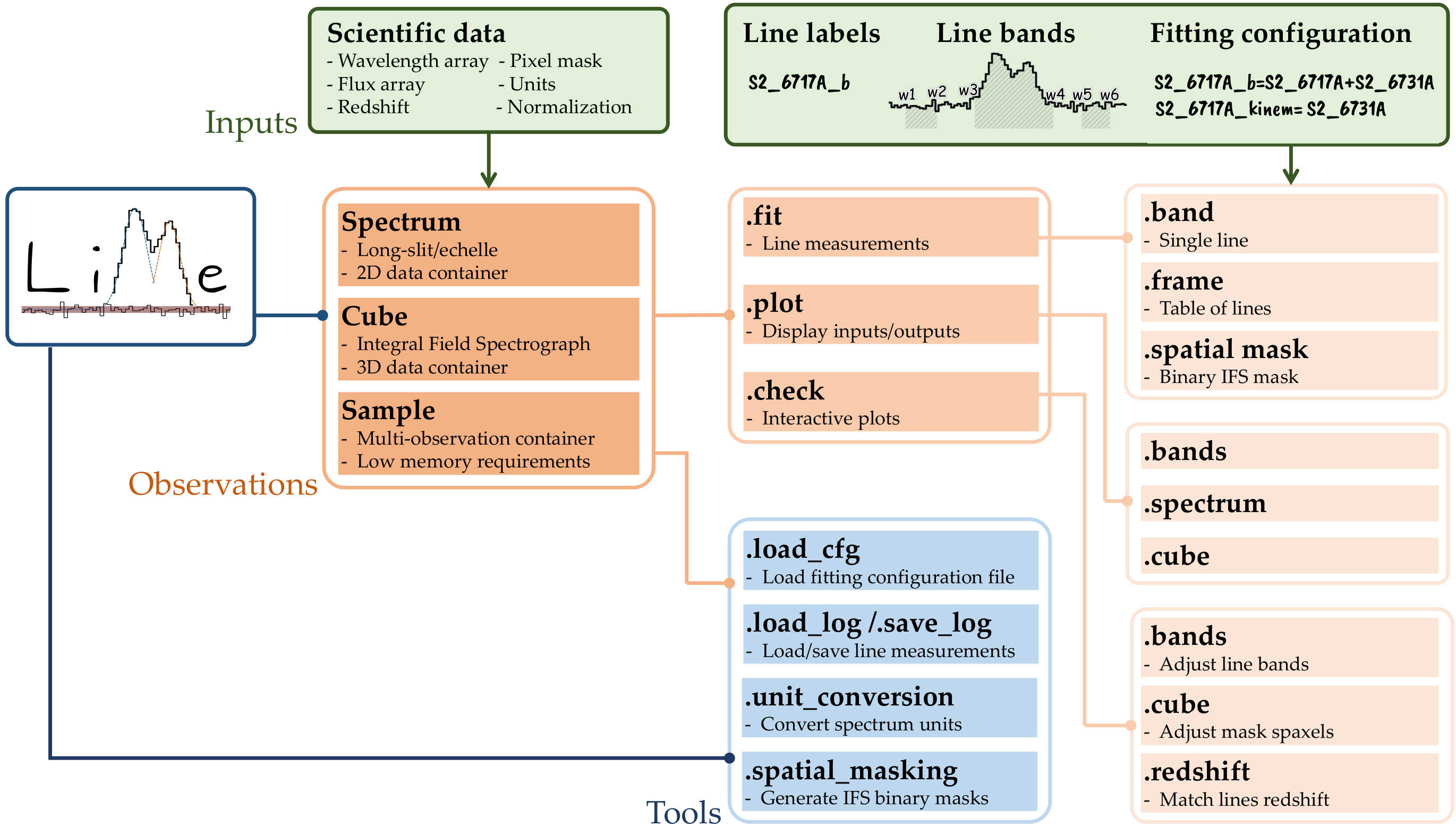
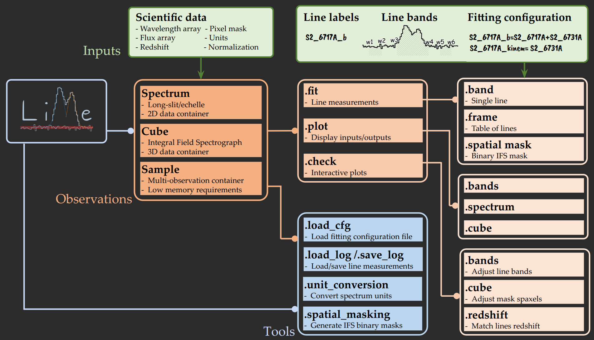
The figure above illustrates the composite design of \(\mathrm{LiMe}\): observations use instances of other classes to organize the available operations.
This modular approach is similar to that of IRAF (see Tody 1986). For example:
The \(\tt{.fit}\) module contains the measurement functions.
The \(\tt{.retrieve}\) module contains the functions that extract or calculate standard variables or parameters from the spectral data.
The \(\tt{.infer}\) module contains the functions that provide more subjective estimates or quantities that can vary depending on the object under study.
The \(\tt{.plot}\) module contains the matplotlib display functions.
The \(\tt{.bokeh}\) module contains the bokeh display functions.
The \(\tt{.check}\) module contains the interactive (matplotlib) plotting functions.
For example, if we load an observation from the examples/0_resources/spectra folder:
import lime
from pathlib import Path


# Locate the data
data_folder = Path('../0_resources/spectra')
sloan_SHOC579 = data_folder/'sdss_dr18_0358-51818-0504.fits'

# Create a spectrum observation
spec = lime.Spectrum.from_file(sloan_SHOC579, instrument='sdss', redshift=0.0479)
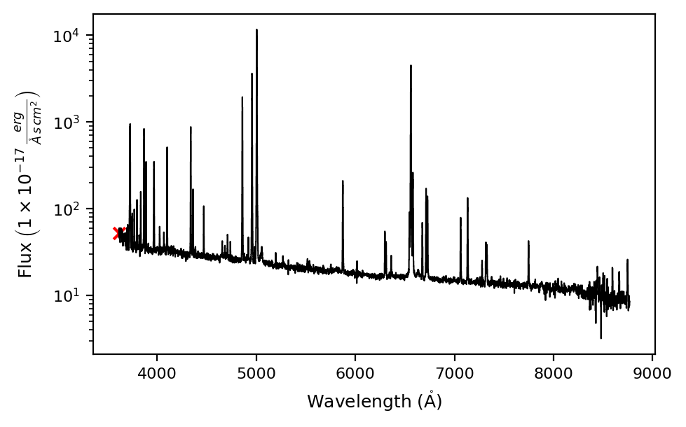
We can plot the spectrum using the \(\tt{.spectrum}\) function in the \(\tt{.plot}\) module:
spec.plot.spectrum(log_scale=True, rest_frame=True)
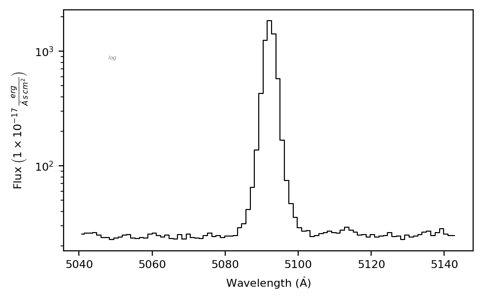
Similarly we can plot a line using \(\tt{.bands}\) function in the same module:
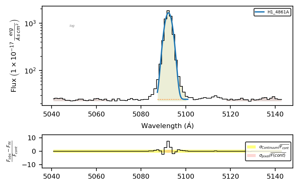
spec.plot.bands('H1_4861A')
Finally, you can a the line using the \(\tt{.band}\) function in the \(\tt{.fit}\) module
spec.fit.bands('H1_4861A', cont_source='adjacent')
If we run \(\tt{plot.bands}\) again we can check the profile:
spec.plot.bands()
Remember: spec.plot.bands() displays the last line in the \(\tt{spec.frame}\) if no labeled is provided.
spec.frame
| wavelength | intg_flux | intg_flux_err | profile_flux | profile_flux_err | eqw | eqw_err | particle | latex_label | group_label | ... | v_10 | v_90 | v_95 | v_99 | chisqr | redchi | aic | bic | observations | comments | |
|---|---|---|---|---|---|---|---|---|---|---|---|---|---|---|---|---|---|---|---|---|---|
| H1_4861A | 4861.25 | 6761.83037 | 43.751246 | 6395.153605 | 253.373325 | 259.322572 | 281.899619 | H1 | $HI4861\mathring{A}$ | none | ... | NaN | NaN | NaN | NaN | 986.415189 | 17.934822 | 170.350792 | 176.532121 | no | no |
1 rows × 74 columns
Takeaways#
The \(\mathrm{LiMe}\) \(\tt{Spectrum}\), \(\tt{Cube}\), and \(\tt{Sample}\) observations match} astronomical spectroscopic datasets.
\(\mathrm{LiMe}\) can create observations directly from the .fits files of certain instruments or by supplying the unpacked data directly. You can read more about these options in the .fits files guide.
Observations provide several functions to measure, plot, and interact with the data. You can find the complete list and their attributes in the API.