%matplotlib widget

Line Bands

The second input in a measurement is the line bands. These are the intervales with the line location and two adjacent and featureless continua. This design was inspired by the the Lick indexes by Worthey et al (1993) and references therein.

This tutorial can be found as a notebook in the Github examples/inputs folder.

Design

The image below shows an example of the bands for the line:

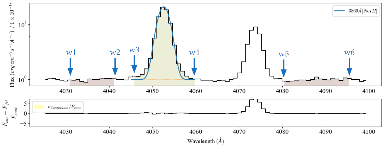
A band consists in a 6-value array with the wavelength boundaries for the line location and two adjacent continua. For measurements, it is essential that:

• The wavelenght array is sorted from lower to higher values.

• The wavelength values are in the rest frame.

• The wavelength units are the same as those declared in the target lime.Spectrum or lime.Cube observations.

Default bands database:

includes a database with common lines which can be observed in astronomical spectra. To access this database you can use the `lime.line_bands <https://lime-stable.readthedocs.io/en/latest/introduction/api.html#lime.line_bands>`__ function:

import numpy as np
from astropy.io import fits
from IPython.display import Image, display
from pathlib import Path
import lime

bands_df = lime.line_bands()

The default table wavelengths are in angstroms with the observed wavelength and band boundaries (w1, w2,w3,w4,w5,w6) values in air for the < < interval

However, you can constrain the output bands from the `lime.line_bands <https://lime-stable.readthedocs.io/en/latest/introduction/api.html#lime.line_bands>`__ function using its attributes. For example, you can limit the output line bands by a wavelenght interval with wave_inter, as well as a lines_list and particle_list. Regarding the output values, you can specify the units_wave and whether to output the vacuum wavelengths via vacuum_conversion=True. Finally, you can state the number of decimals on the line labels using the sig_fig attribute:

lime.line_bands(wave_intvl=(300, 900), particle_list=('He1','O3','S2'), units_wave='nm', decimals=None, vacuum=True)

	wavelength	wave_vac	w1	w2	w3	w4	w5	w6	latex_label	units_wave	particle	transition	rel_int
He1_403nm	402.733452	402.73345	401.503486	402.244991	402.270129	403.335171	403.435647	404.138977	He1-$403nm$	Angstrom	He1	rec	0
S2_407nm	406.974903	406.97490	405.938106	406.587703	406.630488	407.441240	408.159187	408.819158	S2-$407nm$	Angstrom	S2	col	0
O3_436nm	436.443598	436.44360	429.897570	432.494291	435.817822	437.401787	439.206155	441.750863	O3-$436nm$	Angstrom	O3	col	0
He1_447nm	447.274040	447.27404	445.323193	446.639157	446.851915	447.876791	448.209876	449.824056	He1-$447nm$	Angstrom	He1	rec	0
He1_492nm	492.330504	492.33050	490.718146	491.762466	491.908118	492.953284	493.204228	494.116484	He1-$492nm$	Angstrom	He1	rec	0
O3_496nm	496.029500	496.02950	493.073376	494.818947	494.976792	497.217554	497.428449	498.588373	O3-$496nm$	Angstrom	O3	col	0
O3_501nm	500.824004	500.82400	497.326052	498.598165	499.681938	502.578172	502.922278	504.528111	O3-$501nm$	Angstrom	O3	col	0
He1_588nm	587.724329	587.72433	584.742570	586.742789	586.886434	588.729942	589.010016	590.358048	He1-$588nm$	Angstrom	He1	rec	0
He1_668nm	667.999556	667.99955	666.105098	667.204538	667.267813	669.001580	669.174956	670.012944	He1-$668nm$	Angstrom	He1	rec	0
S2_672nm	671.829502	671.82950	668.873329	670.826383	670.941255	672.742554	674.640249	676.192505	S2-$672nm$	Angstrom	S2	col	0
S2_673nm	673.267400	673.26740	668.873329	670.826383	672.741766	674.343008	674.640249	676.192505	S2-$673nm$	Angstrom	S2	col	0
He1_707nm	706.716328	706.71633	703.114524	704.368881	705.727267	708.149955	708.955184	710.651666	He1-$707nm$	Angstrom	He1	rec	0

Using a dataframe:

In , a bands table (and the output line measurement tables) variables are pandas Dataframea.

To get the data from a certain column you can use several commands:

# Table columns
print('Columns', bands_df.columns)

# The index is the first column which is used to index the columns:
labels = bands_df.index.to_numpy()

# Get certain columns
ions = bands_df['particle'].to_numpy()
wave_array = bands_df.wavelength.to_numpy()

# First five values from these columns
print(f"{labels[:5]}, {ions[:5]}, {wave_array[:5]}")

Columns Index(['wavelength', 'wave_vac', 'w1', 'w2', 'w3', 'w4', 'w5', 'w6',
       'latex_label', 'units_wave', 'particle', 'transition', 'rel_int'],
      dtype='object')
['H1_1215A' 'C4_1548A' 'He2_1640A' 'O3_1666A' 'C3_1908A'], ['H1' 'C4' 'He2' 'O3' 'C3'], [1215.1108 1547.6001 1639.7896 1665.5438 1908.0803]

Similarly, you can use these comands to get the data from the rows:

H1_1215A_params = bands_df.iloc[0].to_numpy()
H1_4861A_params = bands_df.loc['H1_4861A'].to_numpy()
print(H1_1215A_params)
print(H1_4861A_params)

[1215.1108 1215.6699 1100.0 1150.0 1195.0 1230.0 1250.0 1300.0
 'H1-$1215\\mathring{A}$' 'Angstrom' 'H1' 'rec' 0]
[4861.2582 4862.691 4809.8 4836.1 4848.715437 4876.181741 4883.13 4908.4
 'H1-$4861\\mathring{A}$' 'Angstrom' 'H1' 'rec' 0]

Finally, you can combine these commands to access the data from certain cells:

bands_df.at['H1_1215A', 'wavelength']

1215.1108

bands_df.loc['H1_1215A', 'wavelength'], bands_df.loc['H1_1215A'].wavelength

(1215.1108, 1215.1108)

bands_df.loc[['H1_1215A', 'H1_4861A'], 'wavelength'].to_numpy(),

(array([1215.1108, 4861.2582]),)

bands_df.loc['H1_1215A':'He2_1640A', 'wavelength'].to_numpy()

array([1215.1108, 1547.6001, 1639.7896])

bands_df.loc['H1_1215A', 'w1':'w6'].to_numpy()

array([1100.0, 1150.0, 1195.0, 1230.0, 1250.0, 1300.0], dtype=object)

Load/save a bands dataframe/measurements log:

To save these dataframes you can use the `save_frame <https://lime-stable.readthedocs.io/en/latest/introduction/api.html#lime.save_log>`__:

# Save to the current folder in several formats:
lime.save_frame('bands_frame.txt', bands_df)
lime.save_frame('bands_frame.pdf', bands_df, parameters=['wavelength', 'latex_label'])

In files with a multi-page structure you can specify the extension:

lime.save_frame('bands_frame.xlsx', bands_df, page='BANDS')
lime.save_frame('bands_frame.fits', bands_df, page='BANDS')

Similarly, to read these files as a pandas dataframe you can use:

bands_df_txt = lime.load_frame('bands_frame.txt')
bands_df_xlsx = lime.load_frame('bands_frame.xlsx', page='BANDS')
bands_df_fits = lime.load_frame('bands_frame.fits', page='BANDS')

Updating the bands database:

The user is adviced to keep his/her own bands database with the bands and latex labels he/she prefers. Afterwards, you can use it in functions (including lime.line_bands) to run your scripts. However, in case you need to update the default database you can recover its location with this command:

lime.io._parent_bands_file

PosixPath('/home/vital/PycharmProjects/lime/src/lime/resources/parent_bands.txt')

Please remember: If you need to update the default lines database make sure to fill all the columns. If there is any issue you can download the default database from the github (or reinstall )