API
Most of  functions can be organized in two categories. In the first one we have the
 Spectrum,
Cube and Sample classes. These functions recreate astronomical observations:
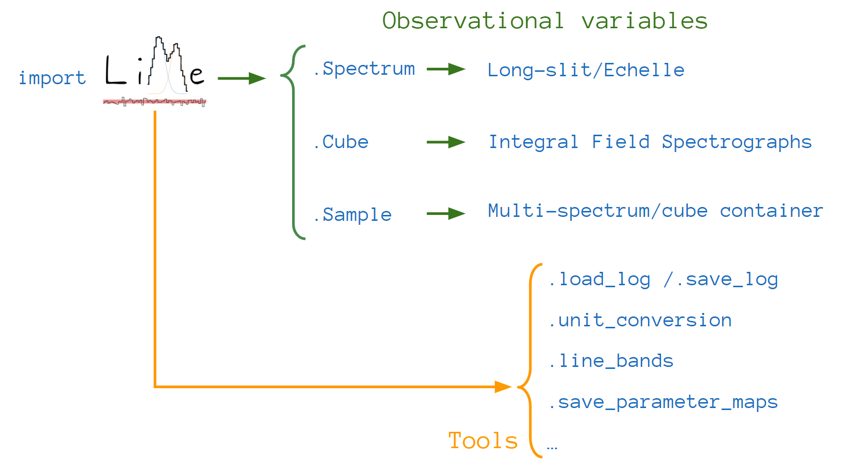
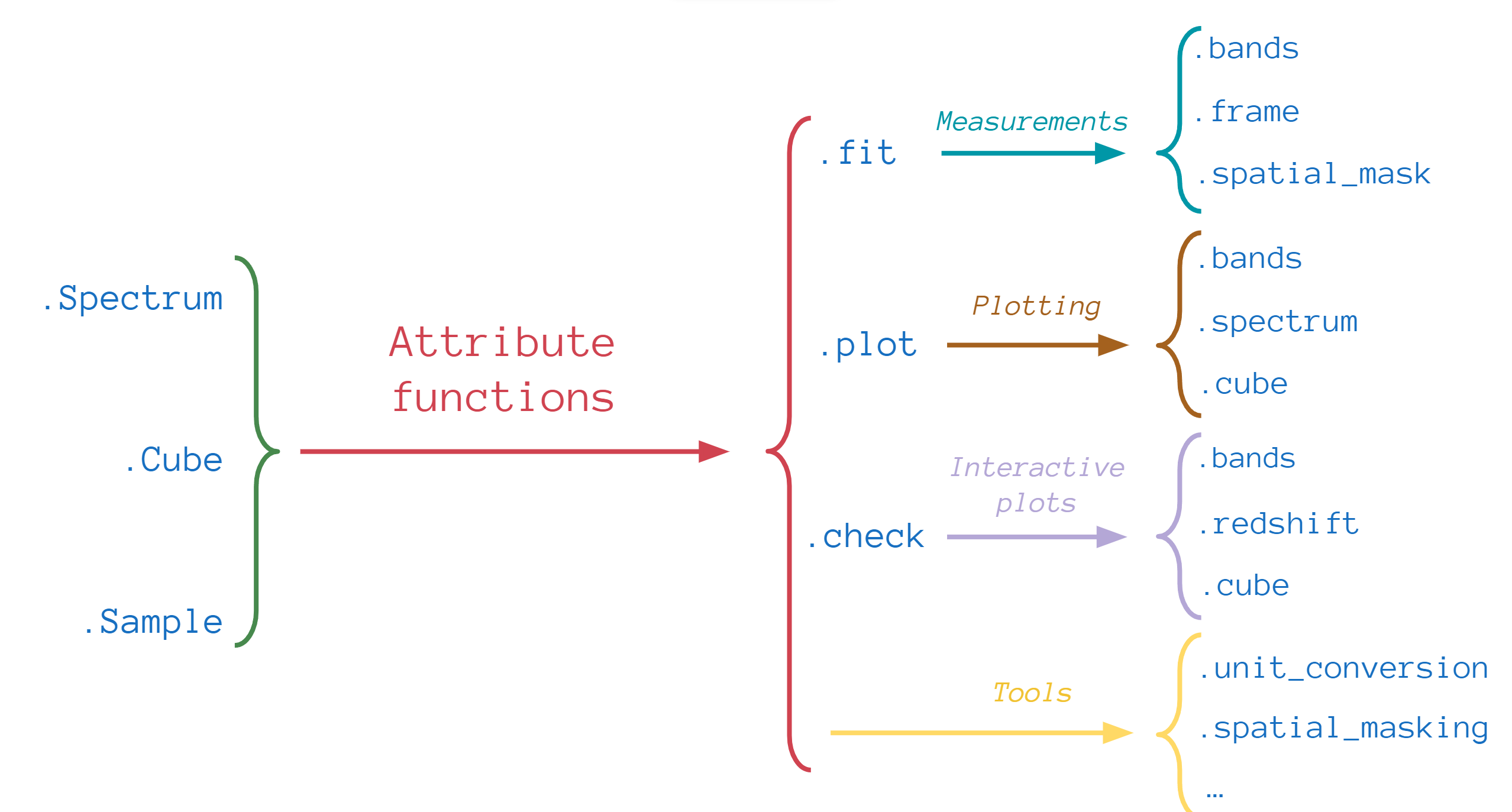
The second set of functions belong to the astronomical objects mentioned above. For example, the .fit, .plot or
.check functions allow us to measure, plot and interact with the data:
Finally, there are additional utility functions. Some of these tools belong to the astronomical objects or they can be
imported directly from or both (as in the case of .load_log/.save_log)
In the following sections we describe these functions and their attributes.
Inputs/outputs
- lime.load_cfg(file_address, fit_cfg_suffix='_line_fitting')[source]
This function reads a configuration file with the toml format. The text file extension must adhere to this format specifications to be successfully read.
If one of the file sections has the suffix specified by the
fit_cfg_suffixthis function will query its items and convert the entries to the format expected by LiMe functions. The default suffix is “_line_fitting”.The function will show a critical warning if it fails to convert an item in a
fit_cfg_suffixsection.- Parameters:
file_address (str, pathlib.Path) – Input configuration file address.
fit_cfg_suffix (str) – Suffix for LiMe configuration sections. The default value is “_line_fitting”.
- Returns:
Parsed configuration data
- Type:
dict
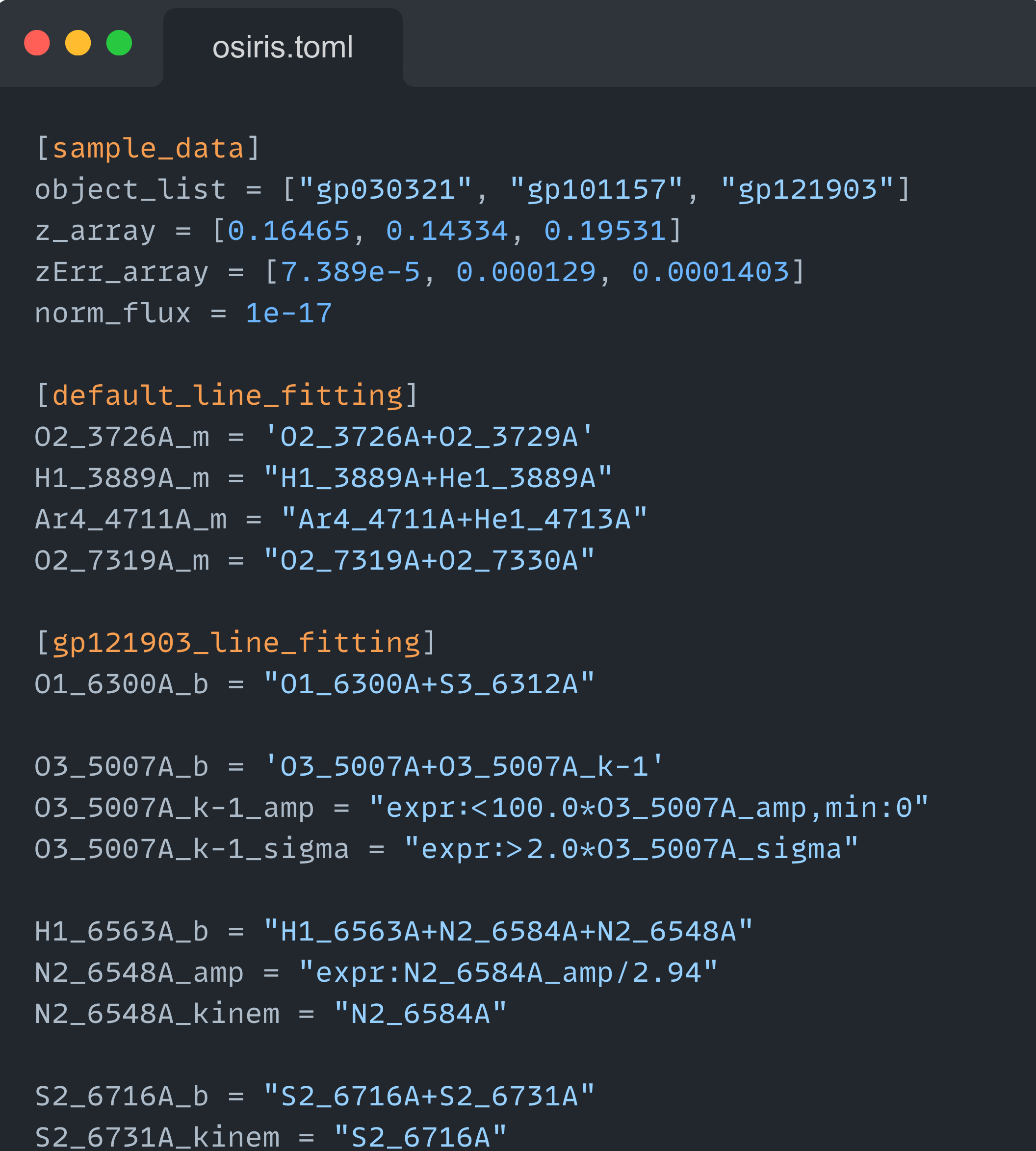
Example of
configuration file
- lime.load_frame(fname, page: str = 'FRAME', levels: list = ['id', 'line'])[source]
This function reads the input
file_addressas a pandas dataframe.The expected file types are “.txt”, “.pdf”, “.fits”, “.asdf” and “.xlsx”. The dataframes expected format is discussed on the line bands and measurements documentation.
For “.fits” and “.xlsx” files the user can provide a page name
extfor the HDU/sheet. The default name is “_LINELOG”.To reconstruct a MultiIndex dataframe the user needs to specify the
sample_levels.- Parameters:
fname (str, Path) – Lines frame file address.
page (str, optional) – Name of the HDU/sheet for “.fits”/”.xlsx” files. The default value is “_LINELOG”.
levels (list, optional) – Indexes name list for MultiIndex dataframes. The default value is [‘id’, ‘line’].
- Returns:
lines log table
- Return type:
pandas.DataFrame
- lime.save_frame(fname, dataframe, page='FRAME', parameters='all', header=None, column_dtypes=None, safe_version=True, **kwargs)[source]
This function saves the input
dataframeat thefnameprovided by the user.The accepted extensions are “.txt”, “.pdf”, “.fits”, “.asdf” and “.xlsx”.
For “.fits” and “.xlsx” files the user can provide a page name for the HDU/sheet with the
extargument. The default name is “FRAME”.The user can specify the
parametersto be saved in the output file.For “.fits” files the user can provide a dictionary to add to the
fits_header. The user can provide acolumn_dtypesstring or dictionary for the output fits file record array. This overwrites LiMe deafult formatting and it must have the same columns as the file names.- Parameters:
fname (str, Path) – Lines frame file address.
dataframe (pandas.DataFrame) – Lines dataframe.
parameters (list) – Output parameters list. The default value is “all”
page (str, optional) – Name of the HDU/sheet for “.fits”/”.xlsx” files.
header (dict, optional) – Dictionary for “.fits” and “.asdf” file headers.
column_dtypes (str, dict, optional) – Conversion variable for the records array <https://pandas.pydata.org/docs/reference/api/pandas.DataFrame.to_records.html>. for the output fits file. If a string or type, the data type to store all columns. If a dictionary, a mapping of column names and indices (zero-indexed) to specific data types.
safe_version (bool, optional) – Save LiMe version as footnote or page header on the output log. The default value is True.
- lime.OpenFits.sdss(fits_address, data_ext_list=(1, 2), hdr_ext_list=0, pixel_mask=None)
This method returns the spectrum array data and headers from a SDSS observation.
The function returns numpy arrays with the wavelength, flux and uncertainty flux (if available this is the standard deviation available), a list with the requested headers and a dictionary with the parameters to construct a LiMe Spectrum. These parameters include the observation wavelength/flux units, normalization and wcs from the input fits file.
- Parameters:
fits_address (int, str or list of either, optional) – File location address for the observation .fits file.
data_ext_list – Data extension number or name to extract from the .fits file.
hdr_ext_list (int, str or list of either, optional) – header extension number or name to extract from the .fits file.
- Returns:
wavelength array, flux array, uncertainty array, header list, observation parameter dict
Tools
- lime.line_bands(wave_intvl=None, lines_list=None, particle_list=None, z_intvl=None, units_wave='Angstrom', decimals=None, vacuum=False, ref_bands=None)[source]
This function returns LiMe bands database as a pandas dataframe.
If the user provides a wavelength array (
wave_inter), a lime.Spectrum or lime.Cube the output dataframe will be limited to the lines within this wavelength interval.Similarly, the user provides a
lines_listor aparticle_listthe output bands will be limited to the these lists. These inputs must follow LiMe notation styleIf the user provides a redshift interval (
z_intvl) alongside the wavelength interval (wave_intvl) the output bands will be limited to the transitions which can be observed given the two parameters.The default line labels and bands
units_waveare angstroms (A), additional options are: um, nm, Hz, cm, mm.The argument
decimalsdetermines the number of decimal figures for the line labels.The user can request the output line labels and bands wavelengths in vacuum setting
vacuum=True. This conversion is done using the relation from Greisen et al. (2006).Instead of the default LiMe database, the user can provide a
ref_bandsdataframe (or the dataframe file address) to use as the reference database.- Parameters:
wave_intvl (list, numpy.array, lime.Spectrum, lime.Cube, optional) – Wavelength interval for output line transitions.
lines_list (list, numpy.array, optional) – Line list for output line bands.
particle_list (list, numpy.array, optional) – Particle list for output line bands.
z_intvl (list, numpy.array, optional) – Redshift interval for output line bands.
units_wave (str, optional) – Labels and bands wavelength units. The default value is “A”.
decimals (int, optional) – Number of decimal figures for the line labels.
vacuum (bool, optional) – Set to True for vacuum wavelength values. The default value is False.
ref_bands (pandas.Dataframe, str, pathlib.Path, optional) – Reference bands dataframe. The default value is None.
- Returns:
- lime.label_decomposition(lines_list, bands=None, fit_conf=None, params_list=('particle', 'wavelength', 'latex_label'), scalar_output=False)[source]
This function takes a
lines_listand returns several arrays with the requested parameters.If the user provides a bands dataframe (
bandsargument) dataframe and a fitting documentation. (fit_confargument) the function will use this information to compute the requested outputs. Otherwise, only the line label will be used to derive the information.The
params_listargument establishes the output parameters arrays. The options available are: “particle”, “wavelength”, “latex_label”, “kinem”, “profile_comp” and “transition_comp”.If the
lines_listargument only has one element the user can request an scalar output withscalar_output=True.- Parameters:
lines_list (list) – Array of lines in LiMe notation.
bands (pandas.Dataframe, str, path.Pathlib, optional) – Bands dataframe (or file address to the dataframe).
fit_conf (dict, optional) – Fitting configuration.
params_list (tuple, optional) – List of output parameters. The default value is (‘particle’, ‘wavelength’, ‘latex_label’)
scalar_output (bool) – Set to True for a Scalar output.
- lime.Spectrum.line_detection(self, bands, sigma_threshold=3, emission_type=True, width_tol=5, band_modification=None, continuum_array=None, continuum_std=None, plot_steps=False)
This function compares the input lines bands in the observation spectrum to confirm the presence of lines.
The input bands can be specified as a pandas dataframe or the path to its file via the
bands_dfargument.The continuum needs to be fit a priori with the Spectrum.fit.continuum function or assigning a
continuum_arrayand acontinuum_std.The
sigma_thresholdestablishes the standard deviation factor beyond which a positive line detection is assumed.By default the algorithm seeks for emission lines, set
emission_typeequal to False for absorption lines.The additional arguments provide additional tools to adjust the line detection and show the steps/results.
- Parameters:
bands (pandas.Dataframe, str, pathlib.Path) – Input bands dataframe or the address to its file.
sigma_threshold (float, optional) – Continuum standard deviation factor for line detection. The default value is 3.
emission_type (str, optional) – Line type. The default value is “True” for emission lines.
width_tol (float, optional) – Minimum number of pixels between peaks/troughs. The default value is 5.
band_modification (str, optional) – Method to adjust the line band with. The default value is None.
ml_detection (str, optional) – Machine learning algorithm to detect lines. The default value is None.
plot_steps (bool, optional) – Plot the detected peaks/troughs. The default value is False
- lime.tools.join_fits_files(log_file_list, output_address, delete_after_join=False, levels=['id', 'line'])[source]
This functions combines multiple log files into single .fits file. The user can request to the delete the individual logs after the individual logs have been combined.
If the case of individual .fits the function loop through the individual HDU and add them to the output file. Currently, this is not available to other multi-page files (such as .xlsx or .asdf)
- Parameters:
log_file_list (list) – Input list of log files.
output_address (bool, optional) – String or path for the output combined log file.
delete_after_join – Delete individual files after joining them. The default value is False
levels (list, optional) – Indexes name list for MultiIndex dataframes. The default value is [‘id’, ‘line’].
- Returns:
- lime.unit_conversion(in_units, out_units, wave_array=None, flux_array=None, dispersion_units=None, decimals=None)[source]
This function converts the input array (wavelength or flux)
in_unitsinto the requestedout_units.Attention
Due to the nature of the
flux_array, the user also needs to include thewave_arrayand its units in thedispersion_units. unitsThe user can also provide the number of
decimalsto round the output array.- Parameters:
in_units (str) – Input array units
out_units (str) – Output array untis
wave_array (numpy.array) – Wavelength array
flux_array (numpy.array) – Flux array
dispersion_units
decimals (int, optional) – Number of decimals.
Astronomical objects
- class lime.Spectrum(input_wave=None, input_flux=None, input_err=None, redshift=None, norm_flux=None, crop_waves=None, inst_FWHM=None, units_wave='AA', units_flux='FLAM', pixel_mask=None, id_label=None, review_inputs=True)[source]
This class creates an astronomical cube variable for an integral field spectrograph observation.
The user needs to provide wavelength and flux arrays. Additionally, the user can include a flux uncertainty array. This uncertainty must be in the same units as the flux. The cube should include its
redshift.If the flux units result in very small magnitudes, the user should also provide a normalization to make the flux magnitude well above zero. Otherwise, the profile fittings are likely to fail. This normalization is removed in the output measurements.
The user can provide a
pixel_maskboolean array with the pixels to be excluded from the measurements.The default
units_waveare angtroms (Å), additional options are: um, nm, Hz, cm, mmThe default
units_fluxare Flam (erg s^-1 cm^-2 Å^-1), additional options are: Fnu, Jy, mJy, nJyThe user can also specify an instrument FWHM (
inst_FWHM), so it can be taken into account during the measurements.The user can provide a
pixel_maskboolean array with the pixels to be excluded from the measurements.- Variables:
fit – Fitting function instance from
lime.workflow.SpecTreatment.plot – Plotting function instance from
lime.plots.SpectrumFigures.
- Parameters:
input_wave (numpy.array) – wavelength array.
input_flux (numpy.array) – flux array.
input_err (numpy.array, optional) – flux sigma uncertainty array.
redshift (float, optional) – observation redshift.
norm_flux (float, optional) – spectrum flux normalization.
crop_waves (np.array, tuple, optional) – spectrum (minimum, maximum) values
inst_FWHM (float, optional) – Instrumental FWHM.
units_wave (str, optional) – Wavelength array units. The default value is “A”.
units_flux (str, optional) – Flux array physical units. The default value is “Flam”.
pixel_mask (np.array, optional) – Boolean array with True values for rejected pixels.
id_label (str, optional) – identity label for the spectrum object
- lime.Spectrum.from_file(file_address, instrument, mask_flux_entries=None, **kwargs)
This method creates a lime.Spectrum object from an observational (.fits) file. The user needs to introduce the file address location and the name of the instrument of survey.
Currently, this method supports NIRSPEC, ISIS, OSIRIS and SDSS as input instrument sources. This method will lower case the input instrument or survey name.
The user can include list of pixel values to generate a mask from the input file flux entries. For example, if the user introduces [np.nan, ‘negative’] the output spectrum will mask np.nan entries and negative fluxes.
This method provides the instrument observational units and normalization but the user should introduce the additional LiMe.Spectrum arguments (such as the observation redshift).
- Parameters:
file_address (Path, string) – Input file location address.
instrument (str) – Input file instrument or survey name
mask_flux_entries (list) – List of pixel values to mask from flux array
kwargs – lime.Spectrum arguments.
- Returns:
lime.Spectrum
- lime.Spectrum.unit_conversion(self, wave_units_out=None, flux_units_out=None, norm_flux=None)
This function converts spectrum wavelength array, the flux array or both arrays units.
The user can also provide a flux normalization for the spectrum flux array.
The wavelength units available are AA (angstroms), um, nm, Hz, cm, mm
The flux units available are Flam (erg s^-1 cm^-2 Å^-1), Fnu (erg s^-1 cm^-2 Hz^-1), Jy, mJy, nJy
- Parameters:
wave_units_out (str, optional) – Wavelength array units
flux_units_out (str, optional) – Flux array units
norm_flux (float, optional) – Flux normalization
- class lime.Cube(input_wave=None, input_flux=None, input_err=None, redshift=None, norm_flux=None, crop_waves=None, inst_FWHM=None, units_wave='AA', units_flux='FLAM', pixel_mask=None, id_label=None, wcs=None)[source]
This class creates an astronomical cube for an integral field spectrograph observation.
The user needs to provide 1D wavelength and 3D flux arrays. Additionally, the user can include a 3D flux uncertainty array. This uncertainty must be in the same units as the flux. The cube should include its
redshift.If the flux units result in very small magnitudes, the user should also provide a normalization to make the flux magnitude well above zero. Otherwise, the profile fittings are likely to fail. This normalization is removed in the output measurements.
The default
units_waveare angtroms (Å), additional options are: um, nm, Hz, cm, mmThe default
units_fluxare Flam (erg s^-1 cm^-2 Å^-1), additional options are: Fnu, Jy, mJy, nJyThe user can also specify an instrument FWHM (
inst_FWHM), so it can be taken into account during the measurements.The user can provide a
pixel_maskboolean 3D array with the pixels to be excluded from the measurements.The observation object should include an astropy World Coordinate System (
wcs) to export the spatial coordinate system to the measurement files.- Parameters:
input_wave (numpy.array) – wavelength 1D array
input_flux (numpy.array) – flux 3D array
input_err (numpy.array, optional) – flux sigma uncertainty 3D array.
redshift (float, optional) – observation redshift.
norm_flux (float, optional) – spectrum flux normalization
crop_waves (np.array, tuple, optional) – spectrum (minimum, maximum) values
inst_FWHM (float, optional) – Instrumental FWHM.
units_wave (str, optional) – Wavelength units. The default value is “A”
units_flux (str, optional) – Flux array physical units. The default value is “Flam”
pixel_mask (np.array, optional) – Boolean 3D array with True values for rejected pixels.
id_label (str, optional) – identity label for the spectrum object
wcs (astropy WCS, optional) – Observation world coordinate system.
- lime.Cube.from_file(file_address, instrument, mask_flux_entries=None, **kwargs)
This method creates a lime.Cube object from an observational (.fits) file. The user needs to introduce the file address location and the name of the instrument of survey.
Currently, this method supports MANGA and MUSE input instrument sources. This method will lower case the input instrument or survey name.
The user can include list of pixel values to generate a mask from the input file flux entries. For example, if the user introduces [“nan”, “negative”] the output spectrum will mask np.nan entries and negative fluxes.
This method procures the instrument observations units, normalization and wcs but the user should introduce the LiMe.Spectrum arguments (such as the observation redshift).
- Parameters:
file_address (Path, string) – Input file location address.
instrument (str) – Input file instrument or survey name
mask_flux_entries (list) – List of pixel values to mask from flux array
kwargs – lime.Cube arguments.
- Returns:
lime.Cube
- lime.Cube.unit_conversion(self, units_wave=None, units_flux=None, norm_flux=None)
This function converts cube wavelength array and/or the flux array units.
The user can also provide a flux normalization for the spectrum flux array.
The wavelength units available are A (angstroms), um, nm, Hz, cm, mm
The flux units available are Flam (erg s^-1 cm^-2 Å^-1), Fnu (erg s^-1 cm^-2 Hz^-1), Jy, mJy, nJy
- Parameters:
units_wave (str, optional) – Wavelength array units
units_flux (str, optional) – Flux array units
norm_flux (float, optional) – Flux normalization
- class lime.Sample(sample_log, levels=('id', 'file', 'line'), load_function=None, instrument=None, folder_obs=None, units_wave='AA', units_flux='FLAM', **kwargs)[source]
This class creates a dictionary-like variable to store LiMe observations, by the fault it is assumed that these are
Spectrumobjects.The sample is indexed via the input
logparameter, a pandas dataframe, whose levels must be declared via thelevelsparameter. By default, three levels are assumed: an “id” column and a “file” column specifying the object ID and observation file address respectively. The “line” level refers to the label measurements in the corresponding The user can specify more levels via thelevelsparameter. However, it is recommended to keep this structure: “id” and “file” levels first and the “line” column last.To create the LiMe observation variables (
SpectrumorCube) the user needs to specify aload_function. This is a python method which declares how the observational files are read and parsed and returns a LiMe object. Thisload_functionmust have 4 parameters:log_df,obs_idx,folder_obsand**kwargs.The first and second variable represent the sample
logand a single pandas multi-index entry for the requested observation. Thefolder_obsand**kwargsare provided at theSamplecreation:The
folder_obsparameter specifies the root file location for the targeted observation file. This root address is combined with the corresponding log levelfilevalue. If afolder_obsis not specified, it is assumed that thefilelog column contains the absolute file address.The
**kwargsargument specifies keyword arguments used in the creation of theSpectrumorCubeobjects such as the`redshiftornorm_fluxfor example.The user may also specify the instrument used for the observation. In this case LiMe will use the inbuilt functions to read the supported instruments. This, however, may not contain all the necessary information to create the LiMe variable (such as the redshift). In this case, the user can include a load_function which returns a dictionary with observation parameters not found on the “.fits” file.
- Parameters:
sample_log (pd.Dataframe) – multi-index dataframe with the parameter properties belonging to the
Sample.levels (list) – levels for the sample log dataframe. By default, these levels are “id”, “file”, “line”.
load_function (python method) – python method with the instructions to convert the observation file into a LiMe observation.
instrument (string, optional.) – instrument name responsible for the sample observations.
folder_obs (string, optional.) – Root address for the observations’ location. This address is combined with the “file” log column value.
kwargs – Additional keyword arguments for the creation of the LiMe observation variables.
- lime.Sample.from_file(id_list, log_list=None, file_list=None, page_list=None, levels=('id', 'file', 'line'), load_function=None, instrument=None, folder_obs=None, **kwargs)
This class creates a dictionary-like variable to store LiMe observations taking a list of observations IDs, line logs and a list of files.
The sample is indexed via the input
logparameter, a pandas dataframe, whose levels must are declared via thelevelsparameter. By default, three levels are assumed: an “id” column and a “file” column specifying the object ID and observation file address respectively. The “line” level refers to the label measurements in the corresponding The user can specify more levels via thelevelsparameter. However, it is recommended to keep this structure: “id” and “file” levels first and the “line” column last.The sample log levels are created from the input values for the
id_list,log_listandfile_listwhile the individual logs from each observation are combined where the line labels in the “line” level. If the input logs are “.fits” files the user must specify extension name or number via thepage_listparameter.To create the LiMe observation variables (
SpectrumorCube) the user needs to specify aload_function. This is a python method which declares how the observational files are read and parsed and returns a LiMe object. Thisload_functionmust have four parameters:log_df,obs_idx,folder_obsand**kwargs.The first and second variable represent the sample
logand a single pandas multi-index entry for the requested observation. Thefolder_obsand**kwargsare provided at theSamplecreation:The
folder_obsparameter specifies the root file location for the targeted observation file. This root address is combined with the corresponding log levelfilevalue. If afolder_obsis not specified, it is assumed that thefilelog column contains the absolute file address. This isThe
**kwargsargument specifies keyword arguments used in the creation of theSpectrumorCubeobjects such as the`redshiftornorm_fluxfor example.- Parameters:
id_list (list) – List of observation names
log_list (list) – List of observation log data frames or files or pandas data frames
file_list (list) – List of observation files.
page_list (list) – List of extension files or names for the observation “.fits” files
levels (list) – levels for the sample log dataframe. By default, these levels are “id”, “file”, “line”.
load_function (python method) – python method with the instructions to convert the observation file into a LiMe observation.
instrument (string, optional.) – instrument name responsible for the sample observations.
folder_obs (string, optional.) – Root address for the observations’ location. This address is combined with the “file” log column value.
kwargs – Additional keyword arguments for the creation of the LiMe observation variables.
Fitting
- lime.workflow.SpecTreatment.bands(self, label, bands=None, fit_conf=None, min_method='least_squares', profile='g-emi', cont_from_bands=True, temp=10000.0, id_conf_prefix=None, default_conf_prefix='default')
This function fits a line on the spectrum object from a given band.
The first input is the line
label. The user can provide a string with the default LiMe notation. Otherwise, the user can provide the transition wavelength in the same units as the spectrum and the transition will be queried from thebandsargument.The second input is the line
bandsthis argument can be a six value array with the same units as the spectrum wavelength specifying the line position and continua location. Otherwise, thebandscan be a pandas dataframe (or the frame address) and the wavelength array will be automatically query from it.If the
bandsare not provided by the user, the default bands database will be used. You can learn more on the bands documentation.The third input is a dictionary the fitting configuration
fit_confattribute. You can learn more on the profile fitting documentation.The
min_methodargument provides the minimization algorithm for the LmFit functions.By default, the profile fitting assumes an emission Gaussian shape, with
profile="g-emi". The profile keywords are described on the label documentationThe
cont_from_bands=Trueargument forces the continuum to be measured from the adjacent line bands. Ifcont_from_bands=Falsethe continuum gradient is calculated from the first and last pixel from the line band (w3-w4)For the calculation of the thermal broadening on the emission lines the user can include the line electron temperature in Kelvin. The default value
tempis 10000 K.- Parameters:
label (str, float, optional) – Line label or wavelength transition to be queried on the
bandsdataframe.bands (np.array, pandas.dataframe, str, Path, optional) – Bands six-value array, bands dataframe (or file address to the dataframe).
fit_conf (dict, optional) – Fitting configuration.
min_method (str, optional) – Minimization algorithm. The default value is ‘least_squares’
profile (str, optional) – Profile type for the fitting. The default value
g-emi(Gaussian-emission).cont_from_bands (bool, optional) – Check for continuum calculation from adjacent bands. The default value is True.
temp (bool, optional) – Transition electron temperature for thermal broadening calculation. The default value is 10000K.
default_conf_prefix (str, optional) – Label for the default configuration section in the
`fit_confvariable.id_conf_prefix (str, optional) – Label for the object configuration section in the
`fit_confvariable.
- lime.workflow.SpecTreatment.frame(self, bands, fit_conf=None, min_method='least_squares', profile='g-emi', cont_from_bands=True, temp=10000.0, line_list=None, default_conf_prefix='default', id_conf_prefix=None, line_detection=False, plot_fit=False, progress_output='bar')
This function measures multiple lines on the spectrum object from a bands dataframe.
The input
bands_dfcan be a pandas.Dataframe or a link to its file.The argument
fit_confprovides the profile-fitting configuration.The
min_methodargument provides the minimization algorithm for the LmFit functions.By default, the profile fitting assumes an emission Gaussian shape, with
profile="g-emi". The profile keywords are described on the label documentationThe
cont_from_bands=Trueargument forces the continuum to be measured from the adjacent line bands. Ifcont_from_bands=Falsethe continuum gradient is calculated from the first and last pixel from the line band (w3-w4).For the calculation of the thermal broadening on the emission lines the user can include the line electron temperature in Kelvin. The default value
tempis 10000 K.The user can limit the fitting to certain bands with the
lines_listargument.If the input
fit_confhas multiple sections, this function will read the parameters from thedefault_conf_keyargument, whose default value is “default”. If the input dictionary also has a section title with theid_conf_label_line_fitting thedefault_conf_key_line_fitting parameters will be updated by the object configuration.If
line_detection=Truethe inputbands_dfmeasurements will be limited to those bands with a line detection. The local configuration for the line detection algorithm can be provided from the fit_conf entries.If
plot_fit=Truethis function will plot profile after each fitting.The
progress_outputargument determines the progress console message. A “bar” value will show a progress bar, while a “counter” value will print a message with the current line being measured. Finally, a None value will not show any message.- Parameters:
bands (pandas.Dataframe, str, path.Pathlib) – Bands dataframe (or file address to the dataframe).
fit_conf (dict, optional) – Fitting configuration.
min_method (str, optional) –
Minimization algorithm. The default value is ‘least_squares’
profile (str, optional) – Profile type for the fitting. The default value
g-emi(Gaussian-emission).cont_from_bands (bool, optional) – Check for continuum calculation from adjacent bands. The default value is True.
temp (bool, optional) – Transition electron temperature for thermal broadening calculation. The default value is 10000K.
line_list (list, optional) – Line list to measure from the bands dataframe.
default_conf_prefix (str, optional) – Label for the default configuration section in the
`fit_confvariable.id_conf_prefix (str, optional) – Label for the object configuration section in the
`fit_confvariable.line_detection (bool, optional) – Set to True to run the dectection line algorithm prior to line measurements.
plot_fit (bool, optional) – Set to True to plot the profile fitting at each iteration.
progress_output (str, optional) – Progress message output. The options are “bar” (default), “counter” and “None”.
- lime.workflow.SpecTreatment.continuum(self, degree_list, emis_threshold, abs_threshold=None, smooth_length=None, plot_steps=False)
This function fits the spectrum continuum in an iterative process. The user specifies two parameters: the
degree_listfor the fitted polynomial and thethreshold_list`for the multiplicative standard deviation factor. At each interation points beyond this flux threshold are excluded from the continuum current fittings. Consequently, the user should aim towards more constrictive parameter values at each iteration.The user can specify a window length over which the spectrum will be smoothed before fitting the continuum using the
smooth_lengthparameter.The user can visually inspect the fitting output graphically setting the parameter
plot_steps=True.- Parameters:
degree_list (list) – Integer list with the degree of the continuum polynomial
emis_threshold (list) – Float list for the multiplicative continuum standard deviation flux factor
smooth_length (integer, optional) – Size of the smoothing window to convolve the spectrum. The default value is None.
plot_steps (bool, optional) – Set to “True” to plot the fitted continuum at each iteration.
- Returns:
- lime.workflow.CubeTreatment.spatial_mask(self, mask_file, output_address, bands=None, fit_conf=None, mask_list=None, line_list=None, log_ext_suffix='_LINELOG', min_method='least_squares', profile='g-emi', cont_from_bands=True, temp=10000.0, default_conf_prefix='default', line_detection=False, progress_output='bar', plot_fit=False, header=None, join_output_files=True)
This function measures lines on an IFS cube from an input binary spatial
mask_file.The results are stored in a multipage “.fits” file, each page contains a measurements and it is named after the spatial array coordinates and the
log_ext_suffix(i.e. “idx_j-idx_i_LINELOG”)The input
bandscan be a pandas.Dataframe or an address to the file. The user can specify one bands file per mask page on themask_file. To do this, thefit_confargument must include a section for every mask on themask_list(i.e. “Mask1_line_fitting”). This function will check for a key “bands” and load the corresponding bands.The fitting configuration in the
fit_confargument accepts a three-level configuration. At the lowest level, Thedefault_conf_keypoints towards the default configuration for all the spaxels analyzed on the cube (i.e. “default_line_fitting”). At an intermediate level, the parameters from the section with a name from themask_list(i.e. “Mask1_line_fitting”) will be applied to the spaxels in the corresponding mask. Finally, at the highest level, the user can provide a spaxel fitting configuration with the spatial array coordiantes “50-28_LINELOG”. In all these cases the higher level configurate updates the lower levels (only common entries are replaced)Attention
In this multi-level configuration design, the higher level entries update the lower level entries: only shared entries are overwritten, the final configuration will include all the entries from the default mask and spaxel sections.
If the
line_detectionis set to True the function proceeds to run the line detection algorithm prior to the fitting of the lines. The user provide the configuration parameters for the line_detection function in thefit_confargument. At the default, mask or spaxel configuration the user needs to specify these entries with the “function name” + “.” + “function argument” (i.e. “line_detection.emission_type=’emission’”). The multi-level configuration described above will be applied to this function parameters as well.Note
The parameters for the
line.detectioncan be found on the documentation. The user doesn’t need to specify a “lime_detection.bands” parameter. The input bands from the corresponding mask will be used.- Parameters:
mask_file (str, pathlib.Path) – Address of binary spatial mask file
output_address (str, pathlib.Path) – File address for the output measurements log.
bands (pandas.Dataframe, str, path.Pathlib) – Bands dataframe (or file address to the dataframe).
fit_conf (dict, optional) – Fitting configuration.
mask_list (list, optional) – Masks name list to explore on the
masks_file.line_list (list, optional) – Line list to measure from the bands dataframe.
log_ext_suffix (str, optional.) – Suffix for the measurements log pages. The default value is “_LINELOG”.
min_method (str, optional) –
Minimization algorithm. The default value is ‘least_squares’
profile (str, optional) – Profile type for the fitting. The default value
g-emi(Gaussian-emission).cont_from_bands (bool, optional) – Check for continuum calculation from adjacent bands. The default value is True.
temp (bool, optional) – Transition electron temperature for thermal broadening calculation. The default value is 10000K.
default_conf_prefix (str, optional) – Label for the default configuration section in the
`fit_confvariable.line_detection (bool, optional) – Set to True to run the dectection line algorithm prior to line measurements.
plot_fit (bool, optional) – Set to True to plot the spectrum lines fitting at each iteration.
progress_output (str, optional) – Progress message output. The options are “bar” (default), “counter” and “None”.
header (dict, optional) – Dictionary for parameter “.fits” file headers.
join_output_files (bool, optional) – In the case of multiple masks, join the individual output “.fits” files into a single one. If set to False there will be one output file named per mask named after it. The default value is True.
Plotting
- lime.plots.SpectrumFigures.spectrum(self, output_address=None, label=None, line_bands=None, rest_frame=False, log_scale=False, include_fits=True, include_cont=False, in_fig=None, fig_cfg={}, ax_cfg={}, maximize=False, detection_band=None)
This function plots the spectrum flux versus wavelength.
The user can include the line bands on the plot if added via the
line_bandsattribute.The user can provide a label for the spectrum legend via the
labelargument.If the user provides an
output_addressthe plot will be stored into an image file instead of being displayed into a window.If the user has installed the library mplcursors, a left-click on a fitted profile will pop-up properties of the fitting, right-click to delete the annotation. This requires
include_fits=True.By default, this function creates a matplotlib figure and axes set to plot the data. However, the user can provide their own
in_figto plot the data. This will return the data-plotted figure object.The default axes and plot titles can be modified via the
ax_cfg. These dictionary keys are “xlabel”, “ylabel” and “title”. It is not necessary to include all the keys in this argument.- Parameters:
output_address (str, optional) – File location to store the plot.
label (str, optional) – Label for the spectrum plot legend. The default label is ‘Observed spectrum’.
line_bands (pd.Dataframe, str, path, optional) – Bands Dataframe (or path to dataframe).
rest_frame (bool, optional) – Set to True for a display in rest frame. The default value is False
log_scale (bool, optional) – Set to True for a display with a logarithmic scale flux. The default value is False
include_fits (bool, optional) – Set to True to display fitted profiles. The default value is False.
include_cont (bool, optional) – Set to True to display fitted continuum. The default value is False.
fig_cfg (dict, optional) – Matplotlib RcParams parameters for the figure format
ax_cfg (dict, optional) – Dictionary with the plot “xlabel”, “ylabel” and “title” values.
in_fig (matplotlib.figure) – Matplotlib figure object to plot the data.
maximize (bool, optional) – Maximise plot window. The default value is False.
- lime.plots.SpectrumFigures.bands(self, line=None, output_address=None, include_fits=True, rest_frame=False, y_scale='auto', fig_cfg=None, ax_cfg=None, in_fig=None, maximize=False)
This function plots a spectrum
line. If alineis not provided the function will select the last line from the measurements log.The user can also introduce a
bandsdataframe (or its file path) to query the inputline.If the user provides an
output_addressthe plot will be stored into an image file instead of being displayed in a window.The
y_scaleargument sets the flux scale for the lines grid. The default “auto” value automatically switches between the matplotlib scale keywords, otherwise the user can set a uniform scale for all.The default axes and plot titles can be modified via the
ax_cfg. These dictionary keys are “xlabel”, “ylabel” and “title”. It is not necessary to include all the keys in this argument.- Parameters:
line (str, optional) – Line label to display.
output_address (str, optional) – File location to store the plot.
include_fits (bool, optional) – Set to True to display fitted profiles. The default value is False.
rest_frame (bool, optional) – Set to True for a display in rest frame. The default value is False
y_scale (str, optional.) – Matplotlib scale keyword. The default value is “auto”.
in_fig (matplotlib.figure) – Matplotlib figure object to plot the data.
fig_cfg (dict, optional) – Dictionary with the matplotlib rcParams parameters .
ax_cfg (dict, optional) – Dictionary with the plot “xlabel”, “ylabel” and “title” values.
maximize (bool, optional) – Maximise plot window. The default value is False.
- Returns:
- lime.plots.SpectrumFigures.grid(self, output_address=None, rest_frame=True, y_scale='auto', n_cols=6, n_rows=None, col_row_scale=(2, 1.5), include_fits=True, in_fig=None, fig_cfg=None, ax_cfg=None, maximize=False)
This function plots the lines from the object spectrum log as a grid.
If the user has installed the library mplcursors, a left-click on a fitted profile will pop-up properties of the fitting, right-click to delete the annotation.
If the user provides an
output_addressthe plot will be stored into an image file instead of being displayed into a window.The default axes and plot titles can be modified via the
ax_cfg. These dictionary keys are “xlabel”, “ylabel” and “title”. It is not necessary to include all the keys in this argument.By default, this function creates a matplotlib figure and axes set to plot the data. However, the user can provide their own
in_figto plot the data. This will return the data-plotted figure object.- Parameters:
output_address (str, pathlib.Path, optional) – Image file address for plot.
rest_frame (bool, optional) – Set to True to plot the spectrum to rest frame. Optional False.
y_scale (str, optional.) – Matplotlib scale keyword. The default value is “auto”.
n_cols (int, optional.) – Number of columns in plot grid. The default value is 6.
n_rows (int, optional.) – Number of rows in plot grid.
col_row_scale (tuple, optional.) – Multiplicative factor for the grid plots width and height. The default value is (2, 1.5).
include_fits (bool, optional) – Set to True to display fitted profiles. The default value is False.
fig_cfg (dict, optional) – Matplotlib RcParams parameters for the figure format
ax_cfg (dict, optional) – Dictionary with the plot “xlabel”, “ylabel” and “title” values.
maximize (bool, optional) – Maximise plot window. The default value is False.
- lime.plots.CubeFigures.cube(self, line, bands=None, line_fg=None, output_address=None, min_pctl_bg=60, cont_pctls_fg=(90, 95, 99), bg_cmap='gray', fg_cmap='viridis', bg_norm=None, fg_norm=None, masks_file=None, masks_cmap='viridis_r', masks_alpha=0.2, wcs=None, fig_cfg=None, ax_cfg=None, in_fig=None, maximise=False)
This function plots the map of a flux band sum for a cube integral field unit observation.
The
lineargument provides the label for the background image. Its bands are read from thebandsargument dataframe. If none is provided, the default lines database will be used to query the bands. Similarly, if the user provides a foregroundline_fgthe plot will include intensity contours from its corresponding band.The user can provide a map baground and foreground contours matplotlib color normalization. Otherwise, a logarithmic normalization will be used.
If the user does not provide a color normalizations at
bg_normandfg_norm. A logarithmic normalization will be used. In this scenariomin_pctl_bgestablishes the minimum flux percentile flux for the background image. The number and separation of flux foreground contours is calculated from the sequence in thecont_pctls_fg.If the user provides the address to a binary fits file to a mask file, this will be overploted on the map as shaded pixels.
- Parameters:
line (str) – Line label for the spatial map background image.
bands (pandas.Dataframe, str, path.Pathlib, optional) – Bands dataframe (or file address to the dataframe).
line_fg (str, optional) – Line label for the spatial map background image contours
output_address (str, optional) – File location to store the plot.
min_pctl_bg (float, optional) – Minimum band flux percentile for spatial map background image. The default value is 60.
cont_pctls_fg (tuple, optional) – Band flux percentiles for foreground
line_fgcontours. The default value is (90, 95, 99)bg_cmap (str, optional) – Background image flux color map. The default value is “gray”.
fg_cmap (str, optional) –
Foreground image flux color map. The default value is “viridis”.
bg_norm (Normalization from matplotlib.colors, optional) – Background image color normalization. The default value is SymLogNorm.
fg_norm (Normalization from matplotlib.colors, optional) –
Foreground contours color normalization. The default value is LogNorm.
masks_file (str, optional) – File address for binary spatial masks
masks_cmap (str, optional) –
Binary masks color map.
masks_alpha (float, optional) – Transparency alpha value. The default value is 0.2 (0 to 1 scale).
wcs (astropy WCS, optional) –
Observation world coordinate system.
fig_cfg (dict, optional) –
Matplotlib RcParams parameters for the figure format
ax_cfg (dict, optional) – Dictionary with the plot “xlabel”, “ylabel” and “title” values.
in_fig (matplotlib.figure) – Matplotlib figure object to plot the data.
maximize (bool, optional) – Maximise plot window. The default value is False.
Interactive plotting
- lime.plots_interactive.BandsInspection.bands(self, bands_file, ref_bands=None, y_scale='auto', n_cols=6, n_rows=None, col_row_scale=(2, 1.5), z_log_address=None, object_label=None, z_column='redshift', fig_cfg=None, ax_cfg=None, in_fig=None, maximize=False)
This function launches an interactive plot from which to select the line bands on the observed spectrum. If this function is run a second time, the user selections won’t be overwritten.
The
bands_fileargument provides to the output database on which the user selections will be saved.The
ref_bandsargument provides the reference database. The default database will be used if none is provided.The
y_scalesets the flux scale for the lines grid. The default “auto” value automatically switches between the matplotlib scale keywords, otherwise the user can set a uniform scale for all.If the user wants to adjust the observation redshift and save the new values the
z_log_addresssets an output dataframe. Theobject_labelandz_columnprovide the row and column indexes to save the new redshift.The default axes and plot titles can be modified via the
ax_cfg. These dictionary keys are “xlabel”, “ylabel” and “title”. It is not necessary to include all the keys in this argument.The online documentation provides more details on the mechanics of this plot function.
- Parameters:
bands_file (str, pathlib.Path) – Output file address for user bands selection.
ref_bands (pandas.Dataframe, str, pathlib.Path, optional) – Reference bands dataframe or its file address. The default database will be used if none is provided.
y_scale (str, optional.) –
Matplotlib scale keywords. The default value is “auto”.
n_cols (int, optional.) – Number of columns in plot grid. The default value is 6.
n_rows (int, optional.) – Number of rows in plot grid.
col_row_scale (tuple, optional.) – Multiplicative factor for the grid plots width and height. The default value is (2, 1.5).
z_log_address (str, pathlib.Path, optional) – Output address for redshift dataframe file.
object_label (str, optional) – Object label for redshift dataframe row indexing.
z_column (str, optional) – Column label for redshift dataframe column indexing. The default value is “redshift”.
fig_cfg (dict, optional) –
Dictionary with the matplotlib rcParams parameters .
ax_cfg (dict, optional) – Dictionary with the plot “xlabel”, “ylabel” and “title” values.
maximize (bool, optional) – Maximise plot window. The default value is False.
- lime.plots_interactive.CubeInspection.cube(self, line, bands=None, line_fg=None, min_pctl_bg=60, cont_pctls_fg=(90, 95, 99), bg_cmap='gray', fg_cmap='viridis', bg_norm=None, fg_norm=None, masks_file=None, masks_cmap='viridis_r', masks_alpha=0.2, rest_frame=False, log_scale=False, fig_cfg=None, ax_cfg_image=None, ax_cfg_spec=None, in_fig=None, lines_file=None, ext_frame_suffix='_LINELOG', wcs=None, maximize=False)
This function opens an interactive plot to display and individual spaxel spectrum from the selection on the image map.
The left-hand side plot displays an image map with the flux sum of a line band as described on the Cube.plot.cube documentation.
A right-click on a spaxel of the band image map will plot the selected spaxel spectrum on the right-hand side plot. This will also mark the spaxel with a red cross.
If the user provides a
masks_filethe plot window will include a dot mask selector. Activating one mask will overplotted on the image band. A middle button click on the image band will add/remove a spaxel to the current pixel selected masks. If the spaxel was part of another mask it will be removed from the previous mask region.If the user provides a
lines_log_file.fits file, the fitted profiles will be included on its corresponding spaxel spectrum plot. The measurements logs on this “.fits” file must be named using the spaxel array coordinate and the suffix on theext_logargument.If the user has installed the library mplcursors, a left-click on a fitted profile will pop-up properties of the fitting, right-click to delete the annotation.
- Parameters:
line (str) – Line label for the spatial map background image.
bands (pandas.Dataframe, str, path.Pathlib, optional) – Bands dataframe (or file address to the dataframe).
line_fg (str, optional) – Line label for the spatial map background image contours
min_pctl_bg (float, optional) – Minimum band flux percentile for spatial map background image. The default value is 60.
cont_pctls_fg (tuple, optional) – Band flux percentiles for foreground
line_fgcontours. The default value is (90, 95, 99)bg_cmap (str, optional) –
Background image flux color map. The default value is “gray”.
fg_cmap (str, optional) –
Foreground image flux color map. The default value is “viridis”.
bg_norm (Normalization from matplotlib.colors, optional) –
Background image color normalization. The default value is SymLogNorm.
fg_norm (Normalization from matplotlib.colors, optional) –
Foreground contours color normalization. The default value is LogNorm.
masks_file (str, optional) – File address for binary spatial masks
masks_cmap (str, optional) –
Binary masks color map.
masks_alpha (float, optional) – Transparency alpha value. The default value is 0.2 (0 to 1 scale).
rest_frame (bool, optional) – Set to True for a display in rest frame. The default value is False
log_scale (bool, optional) – Set to True for a display with a logarithmic scale flux. The default value is False
fig_cfg (dict, optional) –
Matplotlib RcParams parameters for the figure format
ax_cfg_image (dict, optional) – Dictionary with the image band flux plot “xlabel”, “ylabel” and “title” values.
ax_cfg_spec (dict, optional) – Dictionary with the spaxel spectrum plot “xlabel”, “ylabel” and “title” values.
lines_file (str, pathlib.Path, optional) – Address for the line measurements log “.fits” file.
ext_frame_suffix (str, optional) – Suffix for the line measurements log spaxel page name
wcs (astropy WCS, optional) –
Observation world coordinate system.
maximize (bool, optional) – Maximise plot window. The default value is False.