Measurements description
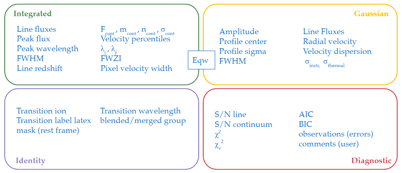
This section describes the parameters measured by  . Unless otherwise noted, these parameters have the same notation
in the output measurements log as the attributes in the programing objects generated with the
. Unless otherwise noted, these parameters have the same notation
in the output measurements log as the attributes in the programing objects generated with the lime.Spectrum class.
These parameter references are also the column names of the pandas.DataFrame lines log (lime.Spectrum.log).
Inputs
This section includes 3 parameters which are actually provided by the user inputs. However, they are also included in the output log for consistency.
line (
.line,str): This attribute is name of the line the measurements belong to. It has the line notation:
format.band (
.band,np.array()): This attribute consists in a six-value vector with the line bands: In thelime.Spectrumobject, the mask is stored as a vector under thelime.Spectrum.maskattribute. In the.logthe wavelengths are stored in individual columns with the headers:w1,w2,w3,w4,w5andw6.profile_label (
.profile_label,str): This attribute consists in a string with the line components separated by dashes (-). The individual components labels have the line notation and they may also have a
suffix for the kinematic component. In single lines, the default value for this attribute is None(string variable). As an example, two profile labels are included below:H1_6563A_b = H1_6563A-H1_6563A_b1-N2_6584A-N2_6548A O2_3727A_m = O2_3727A-O2_3729A
Identification
These parameters are not attributes of the lime.Spectrum class. Nonetheless, they are stored in the lime.Spectrum.log
pandas.DataFrame and the output measuring logs for their convenience in posterior treatments.
wave: This parameter contains the theoretical, rest-frame, wavelength for the emission line. This value is derived from the line label provided by the user.
ion: This parameter contains the ion responsible for the emission line photons. This value is derived from the line label provided by the user.
latex_label: This parameter contains the transition classical notation in latex format. This string includes the profile components if they were provided during the fitting.
Integrated properties
These attributes are calculated by the lime.Spectrum.line_properties function. In these calculations, there is no
assumption on the emission line profile shape.
Attention
In the output measurements log and the lime.Spectrum.log, these parameters have the same flux units as the
input spectrum. However, the attributes of the lime.Spectrum are normalized by the .norm_flux constant
provided by the user at the lime.Spectrum definition.
peak_wave (
.peak_wave,float): This variable is the wavelength of the highest pixel value in the line region.peak_flux (
.peak_flux,float): This variable is the flux of the highest pixel value in the line region.m_cont (
.m_cont,float): Using the line adjacent continua regions fits a linear continuum.
This variable represents is the gradient. y = m*x + nn_cont (
.n_cont,float): Using the line adjacent continua regions fits a linear continuum.
This variable represents is the interception. y = m*x + ncont (
.cont,float): This variable is the flux of the linear continuum at the.peak_wave.cont_err (
.cont_err,float): This variable is standard deviation of the adjacent continua flux. It is calculated from the observed continuum minus the linear model for both continua masks.intg_flux (
.intg_flux,float): This variable contains measurement of the integrated flux. This value is calculated via a Monte Carlo algorithm:If the pixel error spectrum is not provided by the user, the algorithm uses the line
.cont_erras a uniform uncertainty for all the line pixels.The pixel error is added stochastically to each pixel in the line region mask.
The flux in the line region is summed up taking into consideration the line region averaged pixel width and removing the contribution of the linear continuum.
The previous two steps are repeated in a 1000 loop. The mean flux value from the resulting array is taken as the integrated flux value.
intg_err (
.intg_err,float): This attribute contains the integrated flux uncertainty. This value is derived from the standard deviation of the Monte Carlo flux calculation described above.
Attention
Blended components have the same .intg_flux and .intg_err values.
eqw (
.eqw,floatornp.array()): This parameter is the equivalent of the emission line. It is calculated using the expression below: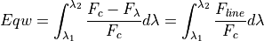
where
 is the integrated flux of the linear continuum in the line region (
.cont) and is the spectrum flux. In single lines,
  is the integrated flux (
.intg_flux) while in blended lines, the corresponding gaussian flux (.gauss_flux) is used. The integration limits for the line region arew3andw4from the input user mask.eqw_err (
.eqw,floatornp.array()): This parameter is the uncertainty in the equivalent width. It is calculated from a Monte Carlo propagation of the.contand its.cont_errand the uncertainty of the line flux.z_line (
.z_line,float): This variable is the emission line redshift: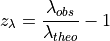
where
 is the
 .peak_wave. In blended lines, this variable is computed using the same.peak_wavefor all transitions (this is the most intense pixel in the line band).FWHM_int (
.FWHM_int,float): This variable is the Full Width Half-Measure in computed from
the integrated profile: The algorithm finds the pixel coordinates which are above half the line peak flux. The blue and and red
edge are subtracted (blue is negative).
computed from
the integrated profile: The algorithm finds the pixel coordinates which are above half the line peak flux. The blue and and red
edge are subtracted (blue is negative).Attention
This operation is only available for lines whose width is above 15 pixels.
snr_line (
.FWHM_int,float): This variable is the signal to noise ratio of the emission line using the definition by Rola et al. 1994: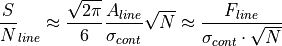
where
 is the amplitude of the line, is the integrated flux of the line (
.intg_flux) is the continuum flux standard deviation (
.cont_err) and is the number of pixels
in the input line band. The later parameter approximates to
is the number of pixels
in the input line band. The later parameter approximates to  in single lines, where
  is the gaussian profile standard deviation.
snr_cont (
.snr_cont,float): This variable is the signal to noise ratio of the emission line region using the formula: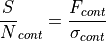
where
is the continuum flux at the peak wavelength and is the continuum flux
standard deviation.v_med (
.v_med,float): This variable is the median velocity of the emission line. The emission line wavelength is converted to velocity units using the formula: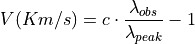
where
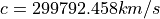 is the speed of light, is the wavelength mask array selection
between
is the speed of light, is the wavelength mask array selection
between  and
and  points and
  is the
 .peak_waveof the emission line.v_50 (
.v_50,float): This variable is velocity corresponding to the 50th percentile of the emission line spectrum where the wavelength array is in. A cumulative sum is performed in the line flux array. Afterwards,
this array is multiplied by the .pixelWidthand divided by the.intg_flux. The resulting vector quantifies the flux percentage corresponding to each pixel in the and mask selection. Afterwards, this vector is
interpolated with respect to the velocity array (whose calculation can be found above).Attention
This operation is only available for lines whose width is above 15 pixels.
v_5 (
.v_5,float): This variable is the velocity corresponding to the 5th percentile of the emission line flux. The calculation procedure is described at the.v_50entry.v_10 (
.v_10,float): This variable is the velocity corresponding to the 10th percentile of the emission line flux. The calculation procedure is described at the.v_50entry.v_90 (
.v_90,float): This variable is the velocity corresponding to the 90th percentile of the emission line flux. The calculation procedure is described at the.v_50entry.v_95 (
.v_95,float): This variable is the velocity corresponding to the 95th percentile of the emission line flux. The calculation procedure is described at the.v_50entry.
Gaussian properties
These attributes are calculated by the lime.Spectrum.gauss_lmfit function. These calculations assume a Gaussian or
multi-Gaussian profile:
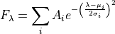
where  is the combined flux profile of the emission line for the line wavelength range
  .
.
 is the height of a gaussian component with respect to the line continuum (
.cont),  is the center
of the of gaussian component and
is the center
of the of gaussian component and  is the standard deviation. The first parameters has the input
flux units (
is the standard deviation. The first parameters has the input
flux units (lime.Spectrum.flux), while the latter two have the input wavelength units (lime.Spectrum.wave).
The output uncertainty in these parameters corresponds to the 1σ error:
This is the standard error which increases the magnitude of the  calculated by the least squares algorithm.
Note
The Gaussian built-in model in LmFit
defines the amplitude  as the flux under the gaussian profile. defines its own model where the
amplitude is defined as the height of the line with respect to the adjacent continuum.
as the flux under the gaussian profile. defines its own model where the
amplitude is defined as the height of the line with respect to the adjacent continuum.
amp (
.amp,np.array()): This array contains the amplitude of the Gaussian profiles. The parameter units are those of the input spectrum flux (lime.Spectrum.flux).amp_err (
.amp_err,np.array()): This array contains the uncertainty on the Gaussian profiles amplitude. The parameter units are those of the input flux (lime.Spectrum.flux).center (
.center,np.array()): This array contains the Gaussian components central wavelength. The parameter units are those of the input spectrum wavelength (lime.Spectrum.wave).center_err (
.center_err,np.array()): This array contains the uncertainty on the Gaussian profiles central wavelength.sigma (
.sigma,np.array()): This array contains the Gaussian components standard deviation. The parameter units are those of the input spectrum wavelength.sigma_err (
.sigma_err,np.array()): This array contains the uncertainty on the Gaussian profiles standard deviation.v_r (
.v_r,np.array()): This array contains the Gaussian components radial velocity in. This
parameter is calculated using the expression: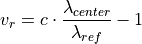
where
is the speed of light,  is the Gaussian profile central wavelength
(
is the Gaussian profile central wavelength
(.center) and is the reference wavelength. In non-blended lines is the
observed peak wavelength (
is the reference wavelength. In non-blended lines is the
observed peak wavelength (.peak_wave). In blended lines, is the component transition wavelength
(.wave) shifted to the observed frame using the redshif provided by the user at thelime.Spectrum.v_r_err (
.v_r_err,np.array()): This array contains the uncertainty of the Gaussian components radial velocity in.sigma_vel (
.sigma_vel,np.array()): This array contains the Gaussian components standard deviation in.
This parameter is calculated using the expression: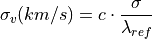
where c
is the speed of light, is the Gaussian profile standard deviation
(.sigma) and is the reference wavelength. In non-blended lines is the
observed peak wavelength (.peak_wave). In blended lines, is the component transition wavelength
(.wave) shifted to the observed frame using the redshif provided by the user at thelime.Spectrum.sigma_vel_err (
sigma_vel_err,floatornp.array()) This array contains the uncertainty of the Gaussian components standard deviation in.FWHM_g (
.FWHM_g,np.array()): This array contains the Full Width Half Maximum of the Gaussian components in in. This parameter is calculated as: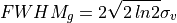
where
is the velocity dispersion of the Gaussian components (.sigma_vel).gauss_flux (
.gauss_flux,np.array()): This array contains the flux of the Gaussian components. It is calculated using the expression: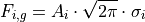
where
 is Gaussian component amplitude (
.amp) and gaussian component standard deviation (.sigma)gauss_flux_err (
.gauss_flux_err,np.array()): This array contains the uncertainty of the Gaussian components flux.
Diagnostics
These section contains the parameters which provide a qualitative or quantitative diagnostic on the line measurement.
chisqr (
.chisqr,float): This variable contains the diagnostic calculated by LmFitredchi (
.redchi,float): This variable contains the reduced diagnostic
calculated by LmFit:
where the
diagnostic is divided by the number of data points, , minus the number of dimensions

aic (
.aic,float): This variable contains the Akaike information criteria calculated by LmFitbic (
.bic,float): This variable contains the Bayesian information criteria calculated by LmFitobservation (
.observation,str): This variable contains errors or warnings generated during the fitting of the line (not implemented).comments (
.comments,str): This variable is left empty for the user to store comments.