[1]:
%matplotlib ipympl
2) Line bands interative inspection
In the previous tutorial, we measured one line from the OSIRIS spectrum of the galaxy GP121903. Before analyzing the full spectrum, however, it is recommended to confirm the presence of lines.
In this tutorial, we are going to compare  lines database with the emission features observed in this spectrum. To do that we are going to use the
 Spectrum.check.bands function to iteratively adjust the observed bands to our observation.
If you are using a jupyter notebook, it is easier to use the %matplotlib ql backend at the top of your notebook, for a better iteration with your plots.
You can download this spectrum from the examples/sample_data. This tutorial can found as a script and a notebook on the examples folder.
Loading the data
Let’s start by importing the script packages and declaring the data location:
[2]:
import numpy as np
from astropy.io import fits
from pathlib import Path
from IPython.display import Image, display
import lime
[3]:
# State the scientific data
obsFitsFile = '../sample_data/spectra/gp121903_osiris.fits'
z_obj = 0.19531
norm_flux = 1e-18
In the first tutorial, we opened the observation using the standard aproach with astropy. This time we are going to use functions to read fits files:
[4]:
gp_spec = lime.Spectrum.from_file(obsFitsFile, instrument='osiris', redshift=z_obj, norm_flux=norm_flux)
From the lime.Spectrum objects we can access the .fit, .plot and .check attributes which organize most of the object functions. For example to plot the spectrum:
[5]:
gp_spec.plot.spectrum(rest_frame=True)
Before measuring the lines, we need to provide their bands. includes a database, which the user can find via the lime.line_bands function:
[6]:
bands_df = lime.line_bands()
[7]:
bands_df
[7]:
| wavelength | wave_vac | w1 | w2 | w3 | w4 | w5 | w6 | latex_label | units_wave | particle | transition | rel_int | |
|---|---|---|---|---|---|---|---|---|---|---|---|---|---|
| H1_1215A | 1215.1108 | 1215.6699 | 1100.0 | 1150.0 | 1195.00000 | 1230.000000 | 1250.0 | 1300.0 | H1-$1215\mathring{A}$ | Angstrom | H1 | rec | 0 |
| C4_1548A | 1547.6001 | 1548.1870 | 1400.0 | 1450.0 | 1530.00000 | 1565.000000 | 1600.0 | 1650.0 | C4-$1548\mathring{A}$ | Angstrom | C4 | rec | 0 |
| He2_1640A | 1639.7896 | 1640.3913 | 1600.0 | 1630.0 | 1635.00000 | 1645.000000 | 1700.0 | 1750.0 | He2-$1640\mathring{A}$ | Angstrom | He2 | rec | 0 |
| O3_1666A | 1665.5438 | 1666.1500 | 1600.0 | 1630.0 | 1660.00000 | 1680.000000 | 1700.0 | 1750.0 | O3-$1666\mathring{A}$ | Angstrom | O3 | col | 0 |
| C3_1908A | 1908.0803 | 1908.7340 | 1870.0 | 1895.0 | 1898.18782 | 1912.243544 | 1930.0 | 1950.0 | C3-$1908\mathring{A}$ | Angstrom | C3 | sem | 0 |
| ... | ... | ... | ... | ... | ... | ... | ... | ... | ... | ... | ... | ... | ... |
| H1_37395A | 37394.7903 | 37405.5500 | 37365.0 | 37385.0 | 37395.00000 | 37415.000000 | 37425.0 | 37440.0 | H1-$37395\mathring{A}$ | Angstrom | H1 | rec | 0 |
| H1_40511A | 40511.0344 | 40522.6900 | 40490.0 | 40500.0 | 40510.00000 | 40535.000000 | 40550.0 | 40570.0 | H1-$40511\mathring{A}$ | Angstrom | H1 | rec | 0 |
| H1_46524A | 46524.3554 | 46537.7400 | 46510.0 | 46515.0 | 46534.00000 | 46546.000000 | 46555.0 | 46575.0 | H1-$46524\mathring{A}$ | Angstrom | H1 | rec | 0 |
| S4_105075A | 105074.7773 | 105105.0000 | 104700.0 | 104900.0 | 105000.00000 | 105200.000000 | 105300.0 | 105500.0 | S4-$105075\mathring{A}$ | Angstrom | S4 | col | 0 |
| S3_187076A | 187076.1931 | 187130.0000 | 186700.0 | 186900.0 | 187100.00000 | 187160.000000 | 187200.0 | 187300.0 | S3-$187076\mathring{A}$ | Angstrom | S3 | col | 0 |
86 rows × 13 columns
The default database covers lines from the ultraviolet to the far infrared. It is more practical to adjust this database to your observational range. You can use your wavelength range lime.Spectrum in the lime.line_bands function (or wavelength limits) to constrain the output lines:
[8]:
bands_df = lime.line_bands(wave_intvl=gp_spec)
[9]:
bands_df
[9]:
| wavelength | wave_vac | w1 | w2 | w3 | w4 | w5 | w6 | latex_label | units_wave | particle | transition | rel_int | |
|---|---|---|---|---|---|---|---|---|---|---|---|---|---|
| Ne5_3426A | 3426.0000 | 3426.0000 | 3390.000000 | 3410.000000 | 3420.000000 | 3430.000000 | 3445.000000 | 3465.000000 | Ne5-$3426\mathring{A}$ | Angstrom | Ne5 | col | 0 |
| H1_3704A | 3703.8013 | 3704.9132 | 3671.309441 | 3681.364925 | 3700.450000 | 3709.100000 | 3758.000000 | 3764.000000 | H1-$3704\mathring{A}$ | Angstrom | H1 | rec | 0 |
| O2_3726A | 3726.0300 | 3727.1000 | 3665.750000 | 3694.260000 | 3716.020000 | 3743.700000 | 3754.880000 | 3767.500000 | O2-$3726\mathring{A}$ | Angstrom | O2 | col | 0 |
| O2_3729A | 3728.8200 | 3729.8600 | 3665.750000 | 3694.260000 | 3716.020000 | 3743.700000 | 3754.880000 | 3767.500000 | O2-$3729\mathring{A}$ | Angstrom | O2 | col | 0 |
| H1_3750A | 3750.0998 | 3751.2244 | 3664.503848 | 3675.720417 | 3746.433569 | 3756.674784 | 3775.220000 | 3792.040000 | H1-$3750\mathring{A}$ | Angstrom | H1 | rec | 0 |
| H1_3771A | 3770.5779 | 3771.7081 | 3759.191222 | 3767.280375 | 3767.467189 | 3775.787336 | 3776.807987 | 3782.905843 | H1-$3771\mathring{A}$ | Angstrom | H1 | rec | 0 |
| H1_3798A | 3797.8450 | 3798.9827 | 3780.949179 | 3792.078244 | 3793.707971 | 3803.676860 | 3807.127865 | 3816.774280 | H1-$3798\mathring{A}$ | Angstrom | H1 | rec | 0 |
| H1_3835A | 3835.3309 | 3836.4789 | 3823.148476 | 3829.538777 | 3831.331855 | 3840.896149 | 3844.260000 | 3852.830000 | H1-$3835\mathring{A}$ | Angstrom | H1 | rec | 0 |
| Ne3_3869A | 3868.7029 | 3869.8600 | 3848.429950 | 3858.099497 | 3862.724063 | 3876.597761 | 3895.538694 | 3910.048413 | Ne3-$3869\mathring{A}$ | Angstrom | Ne3 | col | 0 |
| H1_3889A | 3888.9950 | 3890.1577 | 3842.087829 | 3861.282614 | 3880.390000 | 3899.420000 | 3905.000000 | 3950.000000 | H1-$3889\mathring{A}$ | Angstrom | H1 | rec | 0 |
| H1_3970A | 3970.0170 | 3971.2020 | 3945.566344 | 3957.862489 | 3962.153343 | 3976.592758 | 3979.317175 | 3989.942405 | H1-$3970\mathring{A}$ | Angstrom | H1 | rec | 0 |
| He1_4026A | 4026.1340 | 4027.3345 | 4013.837737 | 4021.250734 | 4021.502052 | 4032.149534 | 4033.154014 | 4040.185370 | He1-$4026\mathring{A}$ | Angstrom | He1 | rec | 0 |
| S2_4069A | 4068.5368 | 4069.7490 | 4058.171690 | 4064.665875 | 4065.093604 | 4073.198887 | 4080.376366 | 4086.974251 | S2-$4069\mathring{A}$ | Angstrom | S2 | col | 0 |
| H1_4102A | 4101.6777 | 4102.8991 | 4084.633589 | 4093.799103 | 4095.935564 | 4108.433334 | 4110.113141 | 4119.294537 | H1-$4102\mathring{A}$ | Angstrom | H1 | rec | 0 |
| H1_4340A | 4340.4035 | 4341.6910 | 4322.549217 | 4332.509864 | 4333.660230 | 4347.675999 | 4350.262697 | 4360.488238 | H1-$4340\mathring{A}$ | Angstrom | H1 | rec | 0 |
| O3_4363A | 4363.1421 | 4364.4360 | 4297.700000 | 4323.660000 | 4356.886082 | 4372.721331 | 4390.760000 | 4416.200000 | O3-$4363\mathring{A}$ | Angstrom | O3 | col | 0 |
| He1_4471A | 4471.4164 | 4472.7404 | 4451.913360 | 4465.069336 | 4467.196330 | 4477.442236 | 4480.772156 | 4496.909458 | He1-$4471\mathring{A}$ | Angstrom | He1 | rec | 0 |
| Fe3_4658A | 4658.0240 | 4659.4000 | 4637.507567 | 4650.238986 | 4653.613936 | 4666.293945 | 4669.709024 | 4679.097970 | Fe3-$4658\mathring{A}$ | Angstrom | Fe3 | col | 0 |
| He2_4685A | 4685.4956 | 4686.8793 | 4663.804252 | 4678.301808 | 4681.274066 | 4691.509985 | 4718.751912 | 4733.650293 | He2-$4685\mathring{A}$ | Angstrom | He2 | rec | 0 |
| Ar4_4711A | 4711.1891 | 4712.5800 | 4664.639652 | 4680.894598 | 4707.992152 | 4720.882185 | 4723.932671 | 4738.660669 | Ar4-$4711\mathring{A}$ | Angstrom | Ar4 | col | 0 |
| Ar4_4740A | 4740.0511 | 4741.4500 | 4605.870000 | 4635.300000 | 4731.467840 | 4748.658238 | 4757.090000 | 4776.100000 | Ar4-$4740\mathring{A}$ | Angstrom | Ar4 | col | 0 |
| H1_4861A | 4861.2582 | 4862.6910 | 4809.800000 | 4836.100000 | 4848.715437 | 4876.181741 | 4883.130000 | 4908.400000 | H1-$4861\mathring{A}$ | Angstrom | H1 | rec | 0 |
| He1_4922A | 4921.8552 | 4923.3050 | 4905.736141 | 4916.176415 | 4917.632529 | 4928.081261 | 4930.590000 | 4939.710000 | He1-$4922\mathring{A}$ | Angstrom | He1 | rec | 0 |
| O3_4959A | 4958.8348 | 4960.2950 | 4929.281844 | 4946.732665 | 4948.310671 | 4970.712011 | 4972.820372 | 4984.416360 | O3-$4959\mathring{A}$ | Angstrom | O3 | col | 0 |
| O3_5007A | 5006.7664 | 5008.2400 | 4971.796688 | 4984.514249 | 4995.348943 | 5024.303156 | 5027.743260 | 5043.797081 | O3-$5007\mathring{A}$ | Angstrom | O3 | col | 0 |
| N2_5755A | 5754.6400 | 5755.0000 | 5700.000000 | 5720.000000 | 5745.000000 | 5765.000000 | 5800.000000 | 5820.000000 | N2-$5755\mathring{A}$ | Angstrom | N2 | col | 0 |
| He1_5876A | 5875.5250 | 5877.2433 | 5845.715833 | 5865.712378 | 5867.148419 | 5885.578291 | 5888.378245 | 5901.854752 | He1-$5876\mathring{A}$ | Angstrom | He1 | rec | 0 |
| O1_6300A | 6300.2076 | 6302.0460 | 6282.963147 | 6293.637954 | 6294.754436 | 6307.155360 | 6319.711710 | 6327.945925 | O1-$6300\mathring{A}$ | Angstrom | O1 | col | 0 |
| S3_6312A | 6311.9682 | 6313.8100 | 6280.559495 | 6295.351299 | 6307.225753 | 6319.552583 | 6321.428405 | 6328.663719 | S3-$6312\mathring{A}$ | Angstrom | S3 | col | 0 |
| N2_6548A | 6547.9514 | 6549.8600 | 6480.030000 | 6520.660000 | 6540.100000 | 6555.950000 | 6627.700000 | 6661.820000 | N2-$6548\mathring{A}$ | Angstrom | N2 | col | 0 |
| H1_6563A | 6562.7192 | 6564.6320 | 6480.030000 | 6520.660000 | 6545.100000 | 6575.950000 | 6627.700000 | 6661.820000 | H1-$6563\mathring{A}$ | Angstrom | H1 | rec | 0 |
| N2_6583A | 6583.3513 | 6585.2700 | 6480.030000 | 6520.660000 | 6575.100000 | 6590.950000 | 6627.700000 | 6661.820000 | N2-$6583\mathring{A}$ | Angstrom | N2 | col | 0 |
| He1_6678A | 6678.0500 | 6679.9955 | 6659.110795 | 6670.102081 | 6670.734647 | 6688.067396 | 6689.800671 | 6698.178167 | He1-$6678\mathring{A}$ | Angstrom | He1 | rec | 0 |
| S2_6716A | 6716.3386 | 6718.2950 | 6686.785257 | 6706.310255 | 6707.458647 | 6725.466528 | 6744.438091 | 6759.956250 | S2-$6716\mathring{A}$ | Angstrom | S2 | col | 0 |
| S2_6731A | 6730.7135 | 6732.6740 | 6686.785257 | 6706.310255 | 6725.458647 | 6741.466528 | 6744.438091 | 6759.956250 | S2-$6731\mathring{A}$ | Angstrom | S2 | col | 0 |
| He1_7065A | 7065.1078 | 7067.1633 | 7029.100000 | 7041.640000 | 7055.220000 | 7079.440000 | 7087.490000 | 7104.450000 | He1-$7065\mathring{A}$ | Angstrom | He1 | rec | 0 |
| Ar3_7136A | 7135.6845 | 7137.7600 | 7099.804897 | 7122.016894 | 7129.546717 | 7145.645711 | 7149.984073 | 7166.354990 | Ar3-$7136\mathring{A}$ | Angstrom | Ar3 | col | 0 |
| O2_7319A | 7318.8124 | 7320.9400 | 7294.873033 | 7310.151519 | 7311.373798 | 7338.569503 | 7340.444100 | 7357.066344 | O2-$7319\mathring{A}$ | Angstrom | O2 | col | 0 |
| O2_7330A | 7329.5494 | 7331.6800 | 7294.873033 | 7310.151519 | 7311.373798 | 7338.569503 | 7340.444100 | 7357.066344 | O2-$7330\mathring{A}$ | Angstrom | O2 | col | 0 |
| Ar3_7751A | 7750.9894 | 7753.2400 | 7731.458685 | 7743.423077 | 7744.234222 | 7759.848767 | 7759.955932 | 7770.429591 | Ar3-$7751\mathring{A}$ | Angstrom | Ar3 | col | 0 |
| H1_8392A | 8392.2696 | 8394.7030 | 8378.449304 | 8387.961949 | 8388.394342 | 8398.627642 | 8398.730000 | 8409.950000 | H1-$8392\mathring{A}$ | Angstrom | H1 | rec | 0 |
| H1_8413A | 8413.1907 | 8415.6300 | 8399.595403 | 8407.110952 | 8410.140000 | 8418.040000 | 8423.876407 | 8432.548195 | H1-$8413\mathring{A}$ | Angstrom | H1 | rec | 0 |
| H1_8438A | 8437.8276 | 8440.2740 | 8396.910000 | 8408.320000 | 8432.872822 | 8443.316230 | 8452.150208 | 8464.463395 | H1-$8438\mathring{A}$ | Angstrom | H1 | rec | 0 |
| H1_8467A | 8467.1263 | 8469.5810 | 8450.080000 | 8459.460000 | 8461.707801 | 8473.595713 | 8474.880000 | 8493.320000 | H1-$8467\mathring{A}$ | Angstrom | H1 | rec | 0 |
| H1_8502A | 8502.3542 | 8504.8190 | 8474.500000 | 8491.730000 | 8499.235520 | 8509.640000 | 8511.060000 | 8533.050000 | H1-$8502\mathring{A}$ | Angstrom | H1 | rec | 0 |
| H1_8545A | 8545.2540 | 8547.7310 | 8515.180000 | 8536.310000 | 8539.268883 | 8552.720348 | 8555.470000 | 8574.470000 | H1-$8545\mathring{A}$ | Angstrom | H1 | rec | 0 |
In addition to the wavelength range, you can also constrain the output table based on a list of ionic species or specify the output units. Check the `line.bands documentation <https://lime-stable.readthedocs.io/en/latest/introduction/api.html#lime.line_bands>`__ to learn all the options available.
A bands dataframe/file consists in a table, where the line bands wavelength limits are stored space-separated columns. The first column has the line label (in the format). The  ,
,  ,
,  ,
,  ,
,  and
and  specify the bands edgets, sorted by increasing wavelengths, for the line location and two adjacent continua:
[10]:
display(Image(filename='../images/bands_definition.png'))
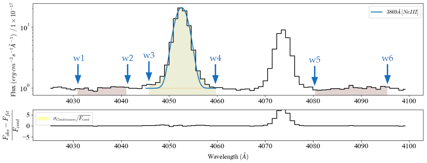
Please remember: The band wavelengths must be on the rest frame and sorted from lower to higher values. Finally, make sure that these wavelengths are in the same units as those from your spectrum.
We can save these bands using lime.save_log function:
[11]:
# Save to a file (if it does not exist already)
bands_df_file = Path('../sample_data/GP121903_bands.txt')
if bands_df_file.is_file() is not True:
    lime.save_frame(bands_df_file, bands_df)
Running the Spectrum.check.bands function opens the interactive window:
[12]:
# Review the bands file
gp_spec.check.bands(bands_df_file)
There are several ways to interact with the plots in this grid: * Right-click on a line sub-plot will remove the line from the output bands file. This will switch the background color to red. * Middle-click on any plot will change the line label suffix on the output bands file. The options are blended (“_b”), merged (“_m”) and single (no suffix) lines. This will change line label the plot title correspondingly. * Left-click and drag allows you to change the bands limits.
In the lattest case, the line or continua bands selections depends on the initical click point. There are some caveats in the window selection: * The plot wavelength range is always 5 pixels beyond the mask bands. Therefore dragging the mouse beyond the mask limits (below w1 or above w6) will change the displayed range. This can be used to move beyond the original wavelength limits. * Selections between the w2 and w5 wavelength bands are always assigned to the line region mask as the new w3 and w4 values. * Due to the previous point, to increase/decrease the the w2 or w5 positions, the user must select a region between w1 and w3 or w4 and w6 respectively.
Each of these adjustments is stored in the input bands_file.
By default, the Spectrum.check.bands function compares the input bands file with the default bands database. Consequently, if you ran the script above again, you will still have your selection. You can provide your own database (file or dataframe) in the parent_bands attribute of the `Spectrum.check.bands function <https://lime-stable.readthedocs.io/en/latest/introduction/api.html#lime.plots_interactive.BandsInspection.bands>`__
At the bottom of the window you can find an slider with the Band (pixels). This slider moves all the bands simultaneously either towards the blue and red limits.
Finally, the Spectrum.check.bands function also gives you the oportunity to seet the effect of the spectrum redshift on the bands selection on a pixel bases and save the new value to a text file (or modify the existing value):
[13]:
# Adding a redshift file address to store the variations in redshift
redshift_file = '../sample_data/redshift_log.txt'
redshift_file_header, object_ref = 'redshift', 'GP121903'
gp_spec.check.bands(bands_df_file, maximize=True, z_log_address=redshift_file, z_column=redshift_file_header,
                    object_label='object_ref')
The new redshift is stored to the output file but the original redshift of the lime.Spectrum does not change (this behaviour shall be changed in a future update).